In this tutorial, we will learn about resampling and feature engineering with the rsample and recipes packages from tidymodels.

Click the button below to clone the course R tutorials into your DataCamp Workspace. DataCamp Workspace is a free computation environment that allows for execution of R and Python notebooks. Note - you will only have to do this once since all tutorials are included in the DataCamp Workspace GBUS 738 project.

Data Resampling

The first step in fitting a machine learning algorithm involves splitting our data into training and test sets as well as processing our data into a numeric feature matrix.

In machine learning, splitting data into training and test sets is known as resampling, or more generally as cross validation. This is an important step in the model fitting process because it allows us to estimate how our trained machine learning algorithms will perform on new data.

The ultimate goal for any machine learning algorithm is to provide accurate predictions on new, previously unseen data.

Resampling is achieved with the rsample package from tidymodels. To demonstrate how this done, let’s import the tidymodels package and the employee_data.

The tidymodels package loads the core machine learning packages that we will be using this semester, including rsample, recipes, parsnip, yardstick, dials, tune, and workflows. Each one of these packages serves a specific role in the modeling process. This tutorial will focus on resampling with rsample and feature engineering with recipes.

library(tidymodels)

── Attaching packages ────────────────────────────────────────────────────────────────────────────────────────────────────────────────────────────────────────────────── tidymodels 1.1.0 ──

✔ broom        1.0.5     ✔ rsample      1.1.1
✔ dials        1.2.0     ✔ tune         1.1.1
✔ infer        1.0.4     ✔ workflows    1.1.3
✔ modeldata    1.1.0     ✔ workflowsets 1.0.1
✔ parsnip      1.1.0     ✔ yardstick    1.2.0
✔ recipes      1.0.6

── Conflicts ───────────────────────────────────────────────────────────────────────────────────────────────────────────────────────────────────────────────────── tidymodels_conflicts() ──
✖ scales::discard()        masks purrr::discard()
✖ dplyr::filter()          masks stats::filter()
✖ recipes::fixed()         masks stringr::fixed()
✖ kableExtra::group_rows() masks dplyr::group_rows()
✖ dplyr::lag()             masks stats::lag()
✖ yardstick::spec()        masks readr::spec()
✖ recipes::step()          masks stats::step()
• Use tidymodels_prefer() to resolve common conflicts.

employee_data <- readRDS(url('https://gmubusinessanalytics.netlify.app/data/employee_data.rds'))

The code below creates a subset of the employee_data with select columns and a new employee_id variable. This is so that we can easily demonstrate the use of the recipes package in the next section.

employee_df <- employee_data %>% 
               select(left_company, job_level, salary, 
                      weekly_hours, miles_from_home)

# View results
employee_df

Data Splitting

The initial_split() function from the rsamplepackage is used for generating a data split object with instructions for randomly assigning rows from a data frame to a training set and test set. Once the object is created, we can use the training() and testing() functions to obtain the two data frames from the object.

When splitting data, it is important to use the set.seed() function before calling initial_split(). The set.seed() function takes any integer as an argument and sets the random number generator in R to a specific starting point. When this is done, the data split will be random the first time our code is executed. Every execution afterwards, will produce the same data split. This guarantees reproducibility.

The initial_split() function takes three important arguments, our data, the proportion of rows to add to our training set (prop), and the variable to use for stratification, strata.

The default prop value is 0.75. The strata argument should contain the outcome variable that we are interesting in predicting. In our case, this is left_company. Stratification ensures that there are an equal proportion of left_company values in the training and test sets.

Creating a Data Split Object

First, let’s create a data split object named employee_split

# Set the random seed
set.seed(314)

employee_split <- initial_split(employee_df, prop = 0.75, 
                                strata = left_company)

If we print the employee_split object, we see that we have 1,103 rows in our training data (known as Analysis in rsample) and 367 rows in the test data (known as Assess in rsample)

employee_split

<Training/Testing/Total>
<1101/369/1470>

Extracting Training and Test Sets

To create training and test data frames from our employee_split object, we must pass employee_split to the training() and testing() functions.

The code below shows how to do this with the %>% operator. I have named the resulting data frames employee_training and employee_test.

When we create the training data, notice that the resulting data frame has 1,103 rows and a random subset of the employees are included.

# Generate a training data frame
employee_training <- employee_split %>% training()

# View results
employee_training

Our test set has 367 rows. Now we are ready to begin our feature engineering steps on the training data.

# Generate a training data frame
employee_test <- employee_split %>% testing()

# View results
employee_test

Feature Engineering

Feature engineering includes all transformations that take a training data set and turn it into a numeric feature matrix.

Typical steps include:

Scaling and centering numeric predictors
Removing skewness from numeric variables
One-hot and dummy variable encoding for categorical variables
Removing correlated predictors and zero variance variables
Imputing missing data

Feature engineering steps should be trained on the training data. This includes things such as learning the means and standard deviations to apply in standardizing numeric predictors.

Once these are calculated in the training data, the same transforms are performed on the test data.

This way, the test data is completely removed from the training process and can serve as an independent assessment for model performance.

Specify a Recipe

The first step in build a feature engineering pipeline with the recipes package is to specify a blueprint for processing data and assigning roles to each column of the training data.

This is done with the recipe() function. This function takes two important arguments:

a model formula
a data frame or tibble for training the recipe

Model formulas in R have the following form:

outcome ~ predictor_1 + predictor_2 + ...

The outcome variable is on the left side of the ~ followed by all predictors separated by a + on the righthand side.

For example, in our employee_training data, we are interested in predicting whether an employee will leave the company. Our response variable is left_company. We would like to use all other variables as predictors. The way to specify this in an R formula is as follows:

left_company ~ job_level + salary + weekly_hours + miles_from_home

Typically, model formulas are written using shorthand notation. When we type left_company ~ ., we are telling R that left_company is the response variable and all other variables should be used as predictors.

This saves us from have to type out each predictor variable separated by a +.

Let’s specify our feature engineering recipe using the employee_training data and the recipe() function. We will name our recipe object employee_recipe

employee_recipe <- recipe(left_company ~ .,
                          data = employee_training)

To explore the variable roles in our recipe, we can pass our recipe object to the summary() function. This will return a data frame with 4 columns. The important columns are variable, type, and role.

The variable column lists all the columns in the input data, employee_training in this case.

The type column lets us know what data type each variable has in our training data.

And finally, the role column specifies the various roles that the recipe() function assigned to each variable based on our model formula.

Notice that since we used left_company ~ . as our formula, the left_company variable is assigned as an outcome variable while all others are assigned as predictor variables.

summary(employee_recipe)

Processing Numeric Variables

Once we have specified a recipe with a formula, data, and correct variables roles, we can add data transformation steps with a series of step() functions. Each step() function in the recipes package provides functionality for different kinds of common transformations.

Centering and Scaling

Let’s begin with the simple task of centering and scaling numeric predictor variables. We have been doing this when we subtracted the mean and divided by the standard deviation in our previous tutorials.

The associated step() functions for this task are step_center() and step_scale(). The step_center() function subtracts the column mean from a variable and step_scale() divides by the standard deviation.

Each successive step() function adds a pre-processing step to our recipe object in the order that they are provided.

All step() functions take a recipe as the first argument, and one or more variables on which to apply the transformation.

There are special selector functions that can be used to select variables by role (outcome or predictor) or type (numeric or nominal).

all_predictors() - select all predictor columns
all_outcomes() - select the outcome variable
all_numeric() - select all numeric columns regardless of role
all_nominal() - select all nominal columns regardless of role

Let’s see what adding these step functions does to our recipe object. We see that we get an updated recipe object as the output with instructions for centering and scaling our numeric columns.

employee_recipe %>% 
  step_center(salary, weekly_hours, miles_from_home) %>% 
  step_scale(salary, weekly_hours, miles_from_home)

But how can we obtain the results of the transformations on our employee_training data frame? We must use the prep() and bake() functions.

The prep() function trains the recipe on a provided dataset and the bake() function applies the prepped recipe to a new data frame of our choice.

Both of these functions take a recipe object as input, so we can chain the commands with a %>% operator.

The code below takes our employee_recipe, adds centering and scaling steps on our numeric predictors, trains the steps with prep() and applies the trained steps to our employee_test data.

The prep() function has a training argument which specifies which data to use for training the pre-processing steps, such as determining the mean and standard deviations of numeric columns for centering and scaling.

The results from bake() will always be a tibble (data frame).

employee_recipe %>% 
  step_center(salary, weekly_hours, miles_from_home) %>% 
  step_scale(salary, weekly_hours, miles_from_home) %>% 
  prep(training = employee_training) %>% 
  bake(new_data = employee_test)

If we wanted to apply our trained recipe to our training data set, it is as simple as updating the new_data argument in bake() to a value of NULL . Since the training data is transformed and a copy is saved during the transformation process in prep(), NULL instructs the bake() function to fetch the results.

Passing new_data = employee_training would also work, but this would re-apply all the transformations to the training data. For small datasets, this doesn’t make a difference. But for large datasets, using NULL can save a lot of time.

employee_recipe %>% 
  step_center(salary, weekly_hours, miles_from_home) %>% 
  step_scale(salary, weekly_hours, miles_from_home) %>% 
  prep(training = employee_training) %>% 
  bake(new_data = NULL)

Using Selector Functions

Instead of specifying the variable names within step() functions, we can use the special selector functions mentioned previously.

In this case, we want to center and scale all numeric predictor variables. We also generally want to exclude processing our outcome variable. In this case, we don’t have to worry about that since our response variable is a factor, but it’s good practice to always exclude the outcome variable with -all_outcomes().

The code below shows how to achieve the previous steps with these special selector functions.

employee_recipe %>% 
  step_center(all_numeric(), -all_outcomes()) %>% 
  step_scale(all_numeric(), -all_outcomes()) %>% 
  prep(training = employee_training) %>% 
  bake(new_data = employee_test)

`step_normalize()`

Centering and scaling numeric predictors is so common that there is one step function, step_normalize(), that does both tasks at once. The code below takes our employee_recipe, adds a normalization step to all numeric predictors except the outcome and id variables, and applies the trained recipe to the employee_test data.

Notice that we get the same results as above.

employee_recipe %>% 
  step_normalize(all_numeric(), -all_outcomes()) %>% 
  prep(training = employee_training) %>% 
  bake(new_data = employee_test)

Transforming Highly Skewed Data

The step_YeoJohnson() function is used to removing skewness in numeric data. This is a special transformation that tries to map the original values of a numeric variable to the normal distribution.

Before we use this function, lets have a look at the distribution of the miles_from_home variable in employee_training.

Note: Another common method for dealing with skewed data is to apply a logarithm transform (usually to base 10). This, however, requires that all numeric data values are greater than zero. The Yeo-Johnson transformation will work on numeric variables that have zero or negative values.

ggplot(data = employee_training, mapping = aes(x = miles_from_home)) +
  geom_histogram(fill = '#006EA1', color = 'white', bins = 10) +
  labs(title = 'Distribution of Miles From Home',
       x = 'Miles from Home',
       y = 'Number of Employees')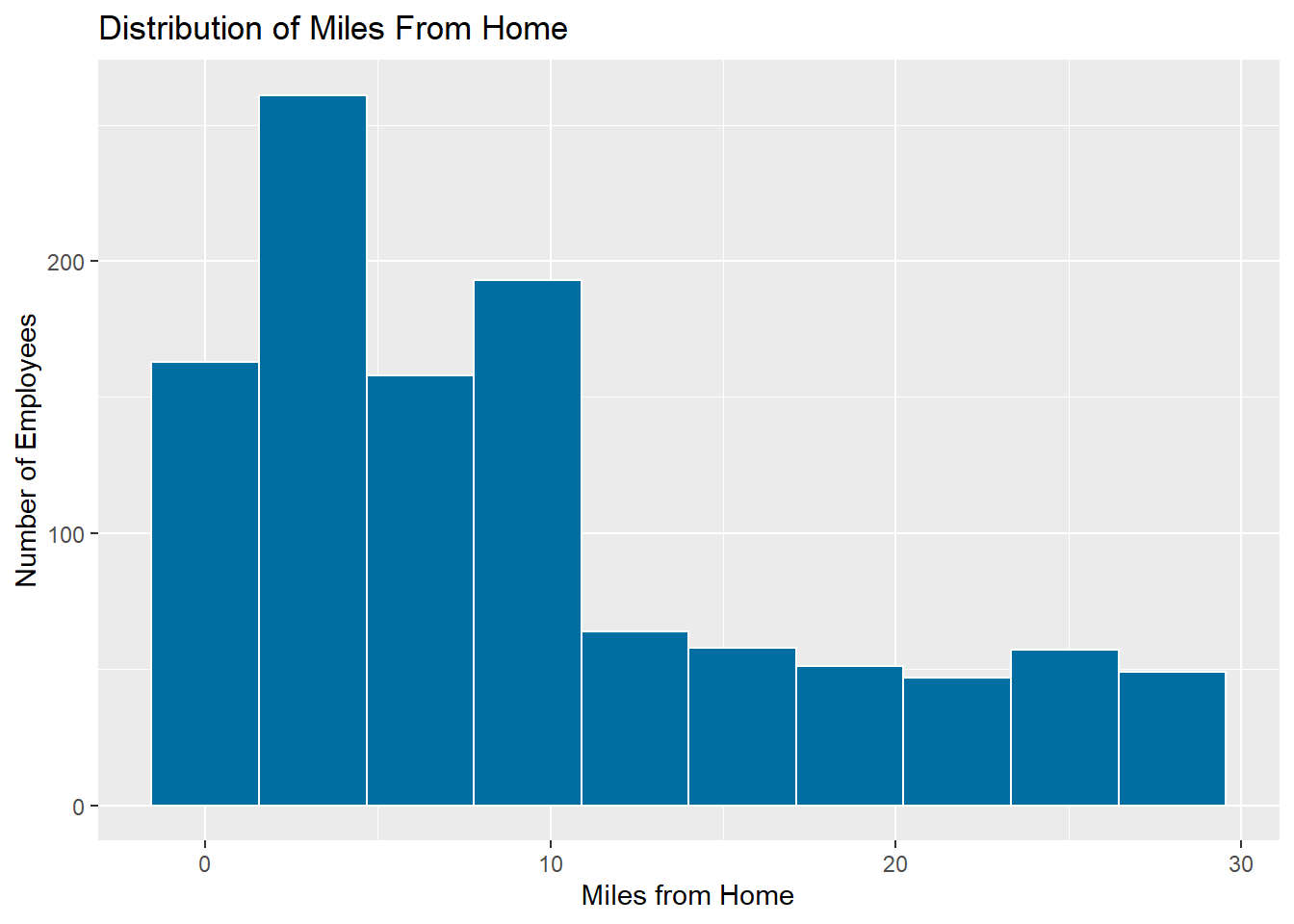

Now let’s transform this variable in the training data with the Yeo-Johnson transformation and look at the resulting values.

employee_recipe %>% 
  step_YeoJohnson(miles_from_home) %>% 
  prep(training = employee_training) %>% 
  bake(new_data = NULL)

Let’s plot the distribution of the results. In the code below, I pipe the results from above into ggplot. Although the results are not perfectly symmetric, they are much better than the original distribution of values. In general, I recommend performing this step on all numeric predictors.

employee_recipe %>% 
  step_YeoJohnson(miles_from_home) %>% 
  prep(training = employee_training) %>% 
  bake(new_data = NULL) %>%
  
  ggplot(mapping = aes(x = miles_from_home)) +
  geom_histogram(fill = '#006EA1', color = 'white', bins = 10) +
  labs(title = 'Distribution of Transformed Miles From Home',
       x = 'Miles from Home',
       y = 'Number of Employees')

Removing Highly Correlated Predictors

Another common feature engineering task is to remove highly correlated predictor variables. High correlation among numeric predictors is known as multicollinearity and can cause trouble in the model fitting process.

To remove correlated numeric predictors, use step_corr(). The step_corr() function has a threshold argument that will remove correlations at that level. The default threshold is set to 0.9. This corresponds to correlations at 0.9 or greater and -0.9 or less.

Let’s use the step_corr() function in on our employee_recipe.

The correlation between salary and weekly_hours in our employee_training data is -0.19. With the default threshold, no variables will be removed. If we change the threshold to 0.15, however, weekly_hours is removed from new data.

# Default threshold of 0.9
employee_recipe %>% 
  step_corr(all_numeric(), -all_outcomes()) %>% 
  prep(training = employee_training) %>% 
  bake(new_data = employee_test)

With a threshold of 0.15, weekly_hours is removed from our new data, employee_test.

employee_recipe %>% 
  step_corr(all_numeric(), -all_outcomes(), threshold = 0.15) %>% 
  prep(training = employee_training) %>% 
  bake(new_data = employee_test)

Putting It All Together

To demonstrate how a full recipe is specified, let’s create a recipe object called employee_numeric that will train the following steps on our employee_training data:

remove highly correlated predictors
remove skewness from all numeric predictors
center and scale all numeric predictors

employee_numeric <- recipe(left_company ~ .,
                           data = employee_training) %>% 
                    step_corr(all_numeric(), -all_outcomes()) %>%  
                    step_YeoJohnson(all_numeric(), -all_outcomes()) %>% 
                    step_normalize(all_numeric(), -all_outcomes()) %>% 
                    prep(training = employee_training)

Now that we have our trained recipe, we can apply the transformations to our training and test data with bake().

processed_employee_training <- employee_numeric %>% 
                               bake(new_data = NULL)

processed_employee_test <- employee_numeric %>% 
                           bake(new_data = employee_test)

# View results
processed_employee_training

# View results
processed_employee_test

Processing Categorical Variables

For a large number of machine learning algorithms, all data in a feature matrix must be numeric. Therefore, any character or factor variables in a data frame must be transformed into numbers.

How is this done? The two primary methods are dummy variable creation and one-hot encoding. Both methods are performed by the step_dummy() function.

Let’s see an example of both methods using our employee_recipe object. We will transform the job_level variable using one-hot encoding and dummy variables.

One-Hot Encoding

The job_level variable in employee_training has 5 unique values: Associate, Manager, Senior Manager, Director, and Vice President.

One-hot encoding will produce 5 new variables that are either 0 or 1 depending on whether the value was present in the job_level row.

The new variables are created with the following naming convention: variable_name_level

For example, job_level_Associate will be one variable that is created. If the value of job_level for any row in the data is “Associate”, then this new variable will be equal to 1 and 0 otherwise.

Let’s see how we can do this with step_dummy()

# One-hot encode job_level
employee_recipe %>% 
  step_dummy(job_level, one_hot = TRUE) %>% 
  prep(training = employee_training) %>% 
  bake(new_data = NULL)

Dummy Variables

Creating dummy variables is similar to one-hot encoding, except that one level is always left out. Therefore, if we create dummy variables from the job_level() function, we will have 4 new variables instead of 5.

This method is generally preferred to one-hot encoding because many statistical models will fail with one-hot encoding. This is because it creates multicollinearity in the one-hot encoded variables.

In fact, the default of step_dummy() is to have one_hot set to FALSE. This is what I recommend for most machine learning applications.

Let’s see the difference when we use the default settings of step_dummy(). Notice that job_level_Associate is now excluded.

employee_recipe %>% 
  step_dummy(job_level) %>% 
  prep(training = employee_training) %>% 
  bake(new_data = NULL)

Creating a Feature Engineering Pipeline

When creating feature engineering recipes with many steps, we have to keep in mind that the transformations are carried out in the order that we enter them.

So if we use step_dummy() before step_normalize() our dummy variables will be normalized because they are numeric at the point when step_normalize() is called.

To make sure we don’t get any unexpected results, it’s best to use the following ordering of high-level transformations:

Correlation filters and skewness transformations - step_YeoJohnson() and step_corr()
Centering, scaling, or normalization on numeric predictors
Dummy variables for categorical data

Let’s put together all that we have learned to create the following feature engineering pipeline on the employee_training data:

Correct for skewness on all numeric predictors
Normalize all numeric predictors
Create dummy variables for all character or factor predictors (we can use the all_nominal() selector for this)

employee_transformations <- recipe(left_company ~ .,
                                   data = employee_training)  %>% 
                            # Transformation steps
                            step_YeoJohnson(all_numeric(), -all_outcomes()) %>%
                            step_normalize(all_numeric(), -all_outcomes()) %>% 
                            step_dummy(all_nominal(), -all_outcomes()) %>% 
                            # Train transformations on employee_training
                            prep(training = employee_training)

# Apply to employee_test
employee_transformations %>% 
  bake(new_data = employee_test)

Resampling and Feature Engineering