Discriminant Analysis and KNN
In this tutorial, we will learn about classification with
discriminant analysis and the K-nearest neighbor (KNN) algorithm. KNN
can be used for both regression and classification and will serve as our
first example for hyperparameter tuning. We will be using two data sets
to demonstrate the algorithms in this lesson, churn_df and
home_sales.
Click the button below to clone the course R tutorials into your DataCamp Workspace. DataCamp Workspace is a free computation environment that allows for execution of R and Python notebooks. Note - you will only have to do this once since all tutorials are included in the DataCamp Workspace GBUS 738 project.
![]()
The code below will load the required packages and data sets for this
tutorial. We will need a new package for this lesson,
discrim. This packages is part of tidymodels
and serves as a general interface to discriminant analysis algorithms in
R.
When installing discrim, you will also need to install
the klaR package.
library(tidymodels)
library(discrim) # for discriminant analysis

# Telecommunications customer churn data
churn_df <- readRDS(url('https://gmubusinessanalytics.netlify.app/data/churn_data.rds'))


# Seattle home sales
home_sales <- readRDS(url('https://gmubusinessanalytics.netlify.app/data/home_sales.rds')) %>%
              select(-selling_date)
Data
We will be working with the churn_df and
home_sales data frames in this lesson.
Take a moment to explore these data sets below.
Telecommunication Customer Churn
A row in this data frame represents a customer at a telecommunications company. Each customer has purchased phone and internet services from this company.
The outcome variable in this data is churn which
indicates whether the customer terminated their services.
Seattle Home Sales
A row in this data frame represents a home that was sold in the Seattle area between 2014 and 2015.
The outcome variable in this data is selling_price.
Linear Discriminant Analysis
Linear discriminant analysis (LDA) is a classification algorithm where the set of predictor variables are assumed to follow a multivariate normal distribution with a common covariance matrix. As we saw in our lecture, this algorithm produces a linear decision boundary.
Both linear and quadratic discriminant analysis can be specified with
the discrim_regularized() function from the
discrim package.
Let’s use LDA to predict whether customers will cancel their
telecommunications service in the churn_df data frame. We
will follow our standard machine learning workflow that was introduced
in the logistic regression tutorial.
Data Splitting
In this case, our event of interest is churn == 'yes'.
This is what we would like to map to the positive class when calculating
our performance metrics.
The code below shows that yes is mapped to the first
level of the churn variable. Since todymodels
maps the first level to the positive class in all performance metrics
functions, we do not need to recode the levels of this variable.
levels(churn_df$churn)[1] "yes" "no"
Now we can proceed to split our data with
initial_split().
set.seed(314) # Remember to always set your seed. Any integer will work

churn_split <- initial_split(churn_df, prop = 0.75,
                             strata = churn)

churn_training <- churn_split %>% training()

churn_test <- churn_split %>% testing()
Feature Engineering
We have a mixture of numeric and factor predictor variables in our
data. We will use step_dummy() to convert all factor
variables to numeric indicator variables.
It is also standard practice to center and scale our numeric
predictors. If needed, we can also adjust for skewness with
step_YeoJohnson().
Let’s make histograms of our numeric predictors to see if this is
needed. We have skewness present in late_payments.
Histograms of numeric predictors
monthly_charges
ggplot(data = churn_df, mapping = aes(x = monthly_charges)) +
  geom_histogram(fill = '#006EA1', color = 'white', bins = 20) +
  labs(title = 'Distribution of Monthly Charges') +
  theme_light()
late_payments
ggplot(data = churn_df, mapping = aes(x = late_payments)) +
  geom_histogram(fill = '#006EA1', color = 'white', bins = 20) +
  labs(title = 'Distribution of Late Payments') +
  theme_light()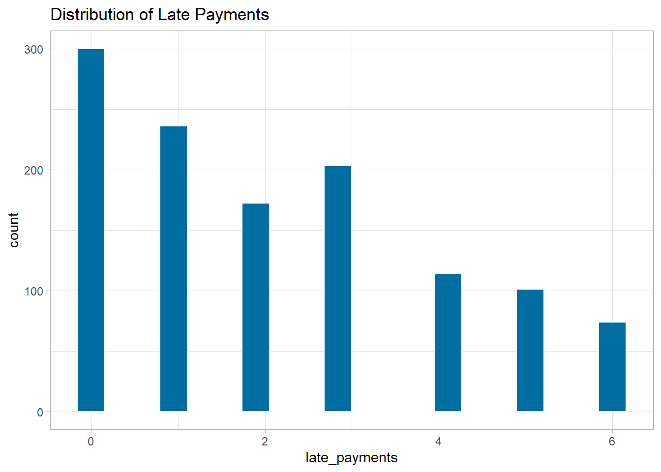
Feature Engineering Recipe
Now we can create a feature engineering recipe for this data. We will train the following transformations on our training data.
- Remove skewness from numeric predictors
- Normalize all numeric predictors
- Create dummy variables for all nominal predictors
churn_recipe <- recipe(churn ~ ., data = churn_training) %>%
                       step_YeoJohnson(all_numeric(), -all_outcomes()) %>%
                       step_normalize(all_numeric(), -all_outcomes()) %>%
                       step_dummy(all_nominal(), -all_outcomes())
Let’s check to see if the feature engineering steps have been carried out correctly.
churn_recipe %>%
  prep(training = churn_training) %>%
  bake(new_data = NULL)
LDA Model Specification
Linear discriminant analysis is specified with the
discrim_regularized function. The optional
frac_common_cov is used to specify an LDA or QDA model.
For LDA, we set frac_common_cov = 1. This instructs
discrim_regularied that we are assuming that each class in
the response variable has the same variance. This is the core assumption
of the LDA model.
FOR QDA, we set frac_common_cov = 0, indicating that
each class within our response variable has its own class-specific
variance.
lda_model <- discrim_regularized(frac_common_cov = 1) %>%
             set_engine('klaR') %>%
             set_mode('classification')
Create a Workflow
Next we create a workflow that combines our feature engineering steps and LDA model.
lda_wf <- workflow() %>%
          add_model(lda_model) %>%
          add_recipe(churn_recipe)
Train and Evaluate With last_fit()
Finally we will train our model and estimate performance on our test
data set using the last_fit() function.
last_fit_lda <- lda_wf %>%
                last_fit(split = churn_split)
To obtain the metrics on the test set (accuracy and roc_auc by
default) we use collect_metrics(). Based on area under the
ROC curve, our model has a “B”.
last_fit_lda %>% collect_metrics()
We can also obtain a data frame with test set results by using the
collect_predictions() function. In the code below, we call
this lda_predictions. It contains the estimated
probabilities for customers canceling their service,
.pred_yes, the predicted class of our response variable,
.pred_class, and the truth, churn.
lda_predictions <- last_fit_lda %>%
                     collect_predictions()

lda_predictions
We can use this data frame to make an ROC plot by using
roc_curve() and autoplot().
lda_predictions %>%
  roc_curve(truth = churn, .pred_yes) %>%
  autoplot()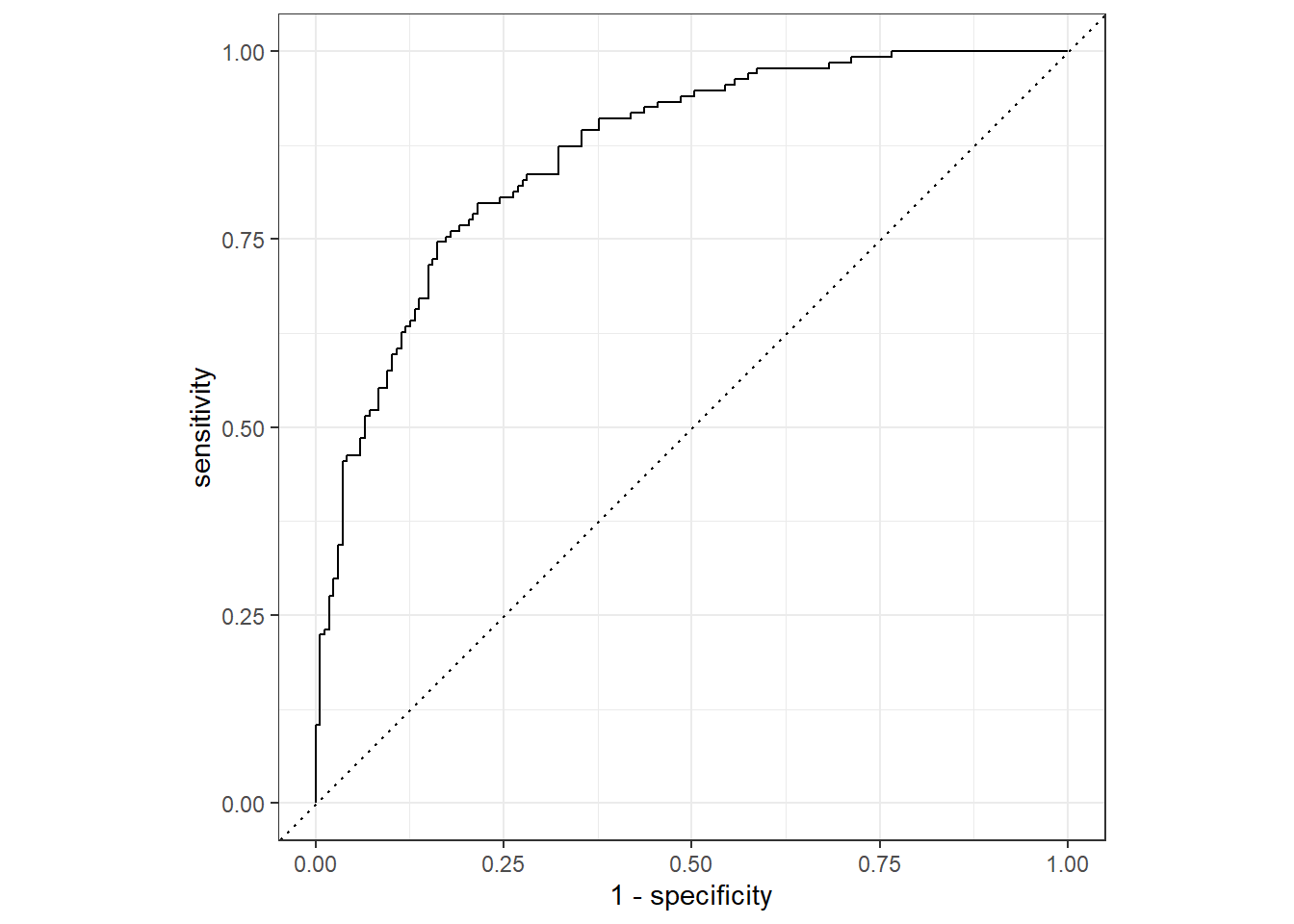
We can also use the lda_predictions results to explore
the confusion matrix and other performance metrics, such as the F1
score, on our test data.
Confusion Matrix
We see that our model made 41 false negatives and 30 false positives. In this case, predicting that a customer will not cancel their service when in fact they do seems like the more costly error.
conf_mat(lda_predictions, truth = churn, estimate = .pred_class) Truth
Prediction yes no
yes 101 30
no 33 137
F1 Score
f_meas(lda_predictions, truth = churn, estimate = .pred_class)
Quadratic Discriminant Analysis
To fit a quadratic discriminant analysis model, we will have to make
some minor adjustments to our workflow from the previous section. We
have already split our data and trained our feature engineering steps so
we only need to create a new QDA model specification with
discrim_regularized() and a new workflow object.
QDA Model Specification
FOR QDA, we set frac_common_cov = 0, indicating that
each class within our response variable has its own class-specific
variance.
qda_model <- discrim_regularized(frac_common_cov = 0) %>%
             set_engine('klaR') %>%
             set_mode('classification')
Create a Workflow
Next we create a QDA workflow object that combines our feature engineering steps from the previous section and our QDA model.
qda_wf <- workflow() %>%
          add_model(qda_model) %>%
          add_recipe(churn_recipe)
Train and Evaluate With last_fit()
Finally we will train our model and estimate performance on our test
data set using the last_fit() function.
last_fit_qda <- qda_wf %>%
                last_fit(split = churn_split)
Based on the area under the ROC curve, our QDA model had similar performance to our LDA model. Remember that QDA is a more complicated model than LDA since we are estimating more parameters.
Since we didn’t get any improvement in terms of model performance, it is always recommended to choose the simpler model if we are deciding which one to use in production.
last_fit_qda %>% collect_metrics()
K-Nearest Neighbor
In this section we will learn how to perform regression and classification using the k-nearest neighbor (KNN) algorithm and hyperparameter tuning with cross validation.
Classification
We will use KNN to predict whether customers will cancel their
service in our chrun_df data. To do this, we have to adjust
our machine learning workflow by incorporating hyperparameter
tuning.
Data Splitting
Since we need to perform hyperparameter tuning, we need to add the
extra step of creating cross validation folds from our training data.
This is done with the vfold_cv() function.
In the code below, we further split our churn_training
data into folds with vfold_cv(). The v
parameter specifies how many folds to create. In our example below, we
are creating 5 folds.
### Create folds for cross validation on the training data set
## These will be used to tune model hyperparameters
set.seed(314)

churn_folds <- vfold_cv(churn_training, v = 5)
Feature Engineering
Since we have already trained our feature engineering steps, we can
use the churn_recipe in our KNN modeling.
KNN Model Specification
The nearest_neighbor() function from the
parnsip package serves as a general interface to KNN
modeling engines in R. It has the following important
hyperparameter:
neighbors- A single integer for the number of neighbors to consider (often called K). For the “kknn” engine, a value of 5 is used if neighbors is not specified
To determine the optimal value of neighbors, we need to
perform hyperparameter tuning. Whenever we have a hyperparameter we
would like to tune, we must set it equal to tune() in our
model specification. In the code below, we specify our KNN
classification model with the “kknn” engine.
knn_model <- nearest_neighbor(neighbors = tune()) %>%
             set_engine('kknn') %>%
             set_mode('classification')
Creating a Workflow
As before the next step is to create a workflow with our recipe and model.
knn_wf <- workflow() %>%
          add_model(knn_model) %>%
          add_recipe(churn_recipe)
Hyperparameter tuning
Hyperparameter tuning is performed using a grid search algorithm. To
do this, we must create a data frame with a column name that matches our
hyperparameter, neighbors in this case, and values we wish
to test.
In the code below we use the tibble() function to create
a data frame with values of neighbors ranging from 10 to
150. Our goal here is to choose a range of values to test, from small to
relatively large numbers of neighbors.
## Create a grid of hyperparameter values to test
k_grid <- tibble(neighbors = c(10, 20, 30, 50, 75, 100, 125, 150))
# View grid
k_grid
Now that we have a data frame with the values of
neighbors to test, we can use the tune_grid()
function to determine the optimal value of our hyperparameter.
The tune_grid() function takes a model or workflow
object, cross validation folds, and a tuning grid as arguments. It is
recommended to use set.seed() before hyperparameter tuning
so that you can reproduce your results at a later time.
## Tune  workflow
set.seed(314)

knn_tuning <- knn_wf %>%
              tune_grid(resamples = churn_folds,
                         grid = k_grid)
To view the results of our hyperparameter tuning, we can use the
show_best() function. We must pass the type of performance
metric we would like to see into the show_best()
function.
From the results below, we see that for each value of
neighbors we specified, tune_grid() fit a KNN
model with that parameter value 5 times (since we have 5 folds in our
cross validation object). The mean column in the results
below indicates the average value of the performance metric that was
obtained.
## Show the top 5 best models based on roc_auc metric
knn_tuning %>% show_best('roc_auc')
We can use the select_best() model to select the model
from our tuning results that had the best overall performance. In the
code below, we specify to select the best performing model based on the
roc_auc metric. We see that the model with 150 neighbors
performed the best.
## Select best model based on roc_auc
best_k <- knn_tuning %>%
          select_best(metric = 'roc_auc')

## View model
best_k
The last step is to use finalize_workflow() to add our
optimal model to our workflow object.
## Finalize workflow by adding the best performing model
final_knn_wf <- knn_wf %>%
                finalize_workflow(best_k)
Train and Evaluate With last_fit()
After we have tuned our hyperparameter, neighbors, and
finalized our workflow object with the optimal model, we perform the
same last steps as before. We will train our model and estimate
performance on our test data set using the last_fit()
function.
last_fit_knn <- final_knn_wf %>%
                last_fit(split = churn_split)
Based on area under the ROC curve, our model has a “B-” and performs slightly worse than LDA and QDA.
last_fit_knn %>% collect_metrics()
ROC Curve
Let’s also have a look at our ROC curve and confusion matrix.
knn_predictions <- last_fit_knn %>%
                   collect_predictions()

knn_predictions
We can use this data frame to make an ROC plot by using
roc_curve() and autoplot().
knn_predictions %>%
  roc_curve(truth = churn, .pred_yes) %>%
  autoplot()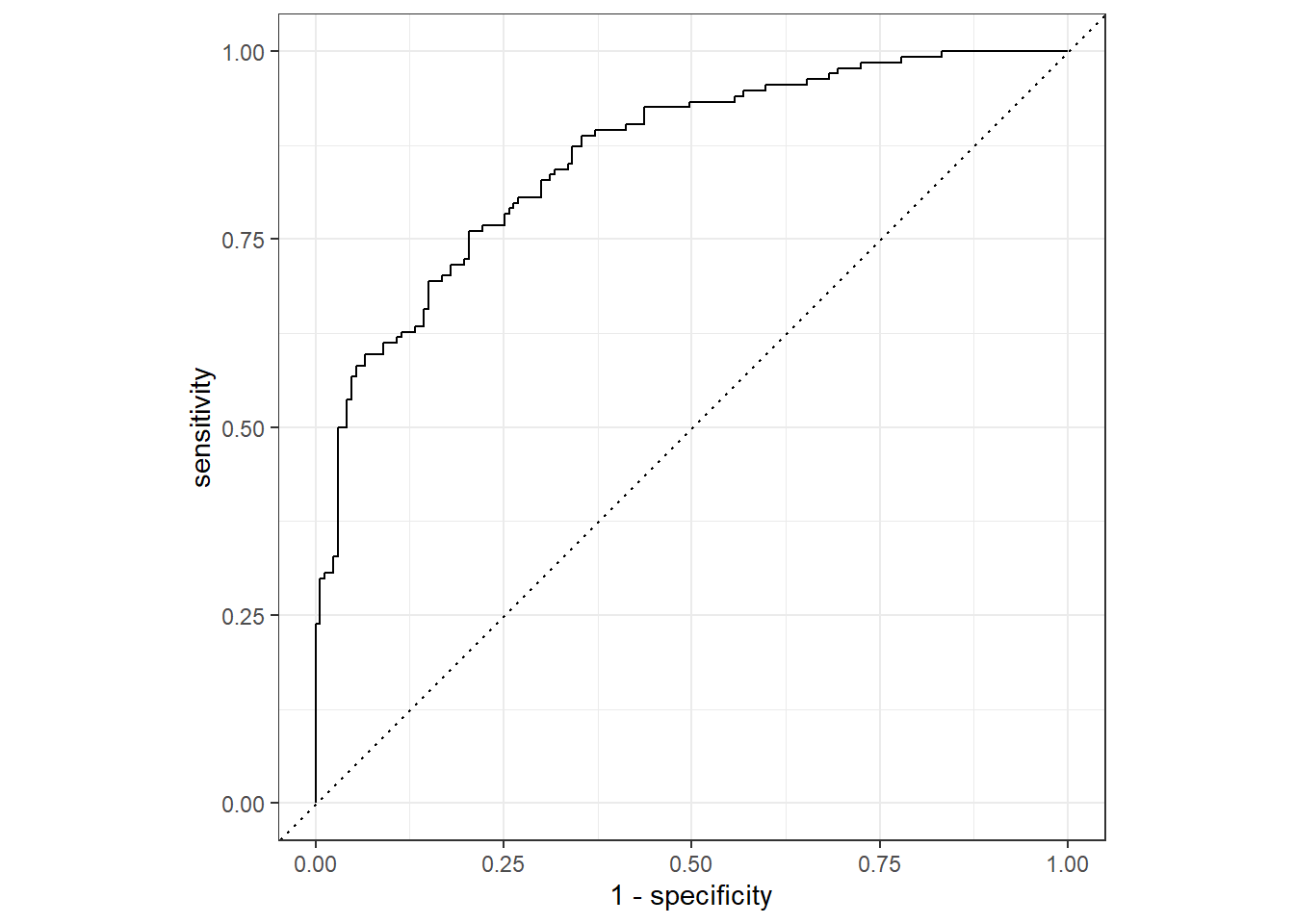
Confusion Matrix
We see that our model made 42 false negatives and 37 false positives.
conf_mat(knn_predictions, truth = churn, estimate = .pred_class) Truth
Prediction yes no
yes 94 29
no 40 138
Regression
In this final section, we will demonstrate a complete machine
learning workflow that incorporates hyperparameter tuning. We will use
KNN to predict the selling price of homes using the
home_sales data.
Data Splitting
First we split our data into training and test sets. We also create 5 cross validation folds from our training data for hyperparameter tuning.
set.seed(271)

# Create a split object
homes_split <- initial_split(home_sales, prop = 0.75,
                             strata = selling_price)

# Build training data set
homes_training <- homes_split %>%
                  training()

# Build testing data set
homes_test <- homes_split %>%
              testing()

## Cross Validation folds
homes_folds <- vfold_cv(homes_training, v = 5)
Feature Engineering
Next, we specify our feature engineering recipe. In this step, we
do not use prep() or bake().
This recipe will be automatically applied in a later step using the
workflow() and last_fit() functions.
For our model formula, we are specifying that
selling_price is our response variable and all others are
predictor variables.
homes_recipe <- recipe(selling_price ~ ., data = homes_training) %>%
                step_YeoJohnson(all_numeric(), -all_outcomes()) %>%
                step_normalize(all_numeric(), -all_outcomes()) %>%
                step_dummy(all_nominal(), - all_outcomes())
As an intermediate step, let’s check our recipe by prepping it on the training data and applying it to the test data. We want to make sure that we get the correct transformations.
From the results below, things look correct.
homes_recipe %>%
  prep(training = homes_training) %>%
  bake(new_data = homes_test)
KNN Regression Model Specification
Next, we specify our KNN regression model with
nearest_neighbor(). We set neighbors to
tune() for hyperparameter tuning and make sure to set the
mode to regression.
knn_reg <- nearest_neighbor(neighbors = tune()) %>%
            set_engine('kknn') %>%
            set_mode('regression')
Create a Workflow
Next, we combine our model and recipe into a workflow object.
knn_reg_wf <- workflow() %>%
              add_model(knn_reg) %>%
              add_recipe(homes_recipe)
Hyperparameter tuning
Let’s test the same values of neighbors as before.
## Create a grid of hyperparameter values to test
k_grid_reg <- tibble(neighbors = c(10, 20, 30, 50, 75, 100, 125, 150))
# View grid
k_grid_reg
Now that we have a data frame with the values of
neighbors to test, we can use the tune_grid()
function to determine the optimal value of our hyperparameter.
The tune_grid() function takes a model or workflow
object, cross validation folds, and a tuning grid as arguments. It is
recommended to use set.seed() before hyperparameter tuning
so that you can reproduce your results at a later time.
## Tune  workflow
set.seed(314)

knn_reg_tuning <- knn_reg_wf %>%
                  tune_grid(resamples = homes_folds,
                            grid = k_grid_reg)
Since we are fitting a regression model, the performance metrics of
interest include rsq and rmse. Let’s use
show_best() to display the best performing model based on
R2
## Show the top 5 best models based on rsq metric
knn_reg_tuning %>% show_best('rsq')
We can use the select_best() model to select the model
from our tuning results that had the best overall performance. In the
code below, we specify to select the best performing model based on the
rsq metric. We see that the model with 20 neighbors
performed the best.
## Select best model based on roc_auc
best_k_reg <- knn_reg_tuning %>%
              select_best(metric = 'rsq')

## View model
best_k_reg
The last step is to use finalize_workflow() to add our
optimal model to our workflow object.
## Finalize workflow by adding the best performing model

final_knn_reg_wf <- knn_reg_wf %>%
                    finalize_workflow(best_k_reg)
Train and Evaluate With last_fit()
Finally, we process our machine learning workflow with
last_fit().
homes_knn_fit <- final_knn_reg_wf %>%
                 last_fit(split = homes_split)
To obtain the performance metrics and predictions on the test set, we
use the collect_metrics() and
collect_predictions() functions on our
homes_knn_fit object.
# Obtain performance metrics on test data
homes_knn_fit %>% collect_metrics()
We can save the test set predictions by using the
collect_predictions() function. This function returns a
data frame which will have the response variables values from the test
set and a column named .pred with the model
predictions.
# Obtain test set predictions data frame
homes_knn_results <- homes_knn_fit %>%
                     collect_predictions()

# View results
homes_knn_results
R2 Plot
Finally, let’s use the homes_knn_results data frame to
make an R2 plot to visualize our model performance on the
test data set. The coord_obs_pred() function will set the x
and y axis scales to be identical and the
scale_*_continuous() functions convert the axis labels to
comma format. This will make the plot easier to interpret.
ggplot(data = homes_knn_results,
       mapping = aes(x = .pred, y = selling_price)) +
  geom_point(alpha = 0.25) +
  geom_abline(intercept = 0, slope = 1, color = 'red', linetype = 2) +
  coord_obs_pred() +
  scale_y_continuous(labels = scales::comma) +
  scale_x_continuous(labels = scales::comma) +
  labs(title = 'KNN Regression Results - Home Sales Test Set',
       x = 'Predicted Selling Price',
       y = 'Actual Selling Price')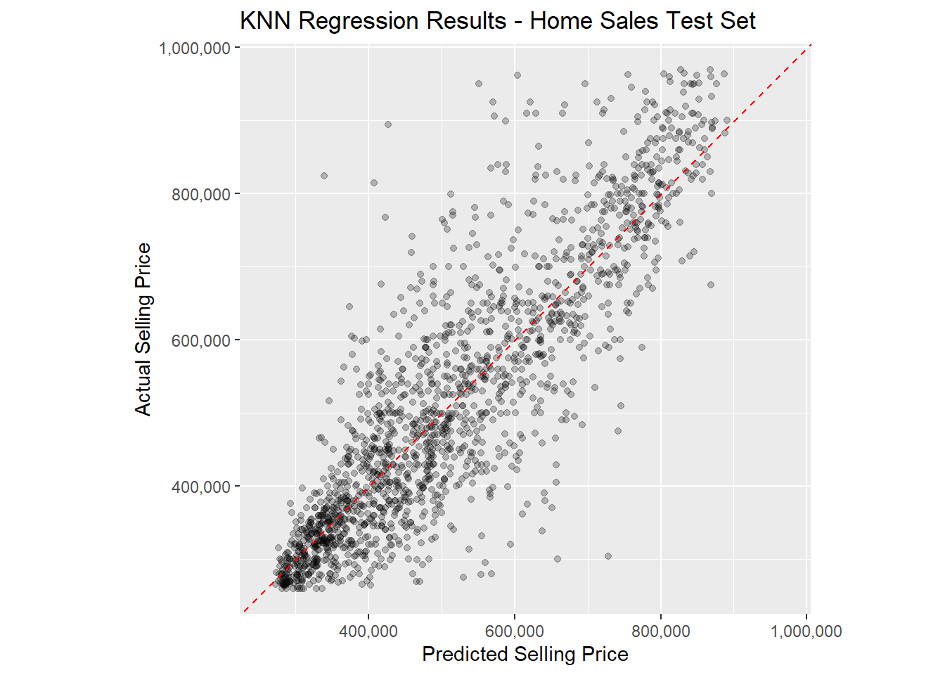
Copyright © David Svancer 2023 |