In this tutorial, we will learn cover decision trees and random forests. These are supervised learning algorithms that can be used for classification or regression.

Click the button below to clone the course R tutorials into your DataCamp Workspace. DataCamp Workspace is a free computation environment that allows for execution of R and Python notebooks. Note - you will only have to do this once since all tutorials are included in the DataCamp Workspace GBUS 738 project.

The code below will load the required packages and data sets for this tutorial. We will need a new package for this lesson, rpart.plot. This packages is used for visualizing decision tree models.

If working with RStudio desktop, please install the rpart, rpart.plot, and ranger packages.

library(tidymodels)
library(vip)
library(rpart.plot)

# Telecommunications customer churn data
churn_df <- readRDS(url('https://gmubusinessanalytics.netlify.app/data/churn_data.rds'))

Data

We will be working with the churn_df data frame in this lesson. Take a moment to explore this data set below.

A row in this data frame represents a customer at a telecommunications company. Each customer has purchased phone and internet services from this company.

The response variable in this data is churn which indicates whether the customer terminated their services.

Decision Trees

To demonstrate fitting decision trees, we will use the churn_df data set and predict churn using all available predictor variables.

A decision tree is specified with the decision_tree() function from tidymodels and has three hyperparameters, cost_complexity, tree_depth, and min_n. Since we will need to perform hyperparameter tuning, we will create cross validation folds from our training data.

Data Splitting

We will split the data into a training and test set. The training data will be further divided into 5 folds for hyperparameter tuning.

set.seed(314) # Remember to always set your seed. Any integer will work

churn_split <- initial_split(churn_df, prop = 0.75, 
                             strata = churn)

churn_training <- churn_split %>% training()

churn_test <- churn_split %>% testing()

# Create folds for cross validation on the training data set
## These will be used to tune model hyperparameters
set.seed(314)

churn_folds <- vfold_cv(churn_training, v = 5)

Feature Engineering

Now we can create a feature engineering recipe for this data. We will train the following transformations on our training data.

Remove skewness from numeric predictors
Normalize all numeric predictors
Create dummy variables for all nominal predictors

churn_recipe <- recipe(churn ~ ., data = churn_training) %>% 
                       step_YeoJohnson(all_numeric(), -all_outcomes()) %>% 
                       step_normalize(all_numeric(), -all_outcomes()) %>% 
                       step_dummy(all_nominal(), -all_outcomes())

Let’s check to see if the feature engineering steps have been carried out correctly.

churn_recipe %>% 
  prep(training = churn_training) %>% 
  bake(new_data = NULL)

Model Specification

Next, we specify a decision tree classifier with the following hyperparameters:

cost_complexity: The cost complexity parameter (a.k.a. C_p or \(\lambda\))
tree_depth: The maximum depth of a tree
min_n: The minimum number of data points in a node that are required for the node to be split further.

To specify a decision tree model with tidymodels, we need the decision_tree() function. The hyperparameters of the model are arguments within the decision_tree() function and may be set to specify values.

However, if tuning is required, then each of these parameters must be set to tune().

We will be using the rpart engine since it will allow us to easily make plots of our decision tree models with the rpart.plot() function.

tree_model <- decision_tree(cost_complexity = tune(),
                            tree_depth = tune(),
                            min_n = tune()) %>% 
              set_engine('rpart') %>% 
              set_mode('classification')

Workflow

Next, we combine our model and recipe into a workflow to easily manage the model-building process.

tree_workflow <- workflow() %>% 
                 add_model(tree_model) %>% 
                 add_recipe(churn_recipe)

Hyperparameter Tuning

We will perform a grid search on the decision tree hyperparameters and select the best performing model based on the area under the ROC curve during cross validation.

For models with multiple hyperparameters, tidymodels has the grid_regular() function for automatically creating a tuning grid with combinations of suggested hyperparameter values.

The grid_regular() function takes the hyperparameters as arguments and a levels option. The levels option is used to determine the number of values to create for each unique hyperparameter.

The number of rows in the grid will be # levels^{# hyperparameters}

For example, with levels = 2 and 3 model hyperparameters, the grid_regular() function will produce a tuning grid with 2³ = 8 hyperparameter combinations.

See the example below, where we create the tree_grid object.

## Create a grid of hyperparameter values to test
tree_grid <- grid_regular(cost_complexity(),
                          tree_depth(),
                          min_n(), 
                          levels = 2)

# View grid
tree_grid

An equivalent way of building tuning grids is by using the parameters() function. When we pass a parsnip model object with tune parameters into the parameters() function, it will automatically extract them.

tree_grid <- grid_regular(parameters(tree_model), 
                          levels = 2)

tree_grid

Tuning Hyperparameters with `tune_grid()`

To find the optimal combination of hyperparameters from our tuning grid, we will use the tune_grid() function.

As in the our KNN example, this function takes a model object or workflow as the first argument, cross valdidation folds for the second, and a tuning grid data frame as the third argument.

It is always sugguested to use set.seed() before using tune_grid() in order to be able to reproduce the results at a later time.

## Tune decision tree workflow
set.seed(314)

tree_tuning <- tree_workflow %>% 
               tune_grid(resamples = churn_folds,
                         grid = tree_grid)

To view the results of our hyperparameter tuning, we can use the show_best() function. We must pass the type of performance metric we would like to see into the show_best() function.

From the results below, we see that for each combination of hyperparameters in our grid, tune_grid() fit a decision tree model with that combination 5 times (since we have 5 folds in our cross validation object).

The mean column in the results below indicates the average value of the performance metric that was obtained.

## Show the top 5 best models based on roc_auc metric
tree_tuning %>% show_best('roc_auc')

We can use the select_best() model to select the model from our tuning results that had the best overall performance. In the code below, we specify to select the best performing model based on the roc_auc metric.

We see that the model with a cost complexity of 1^-10, a tree depth of 15, and minimum n of 40 produced the best model.

## Select best model based on roc_auc
best_tree <- tree_tuning %>% 
             select_best(metric = 'roc_auc')

# View the best tree parameters
best_tree

Finalize Workflow

The last step in hyperparameter tuning is to use finalize_workflow() to add our optimal model to our workflow object.

final_tree_workflow <- tree_workflow %>% 
                       finalize_workflow(best_tree)

Visualize Results

In order to visualize our decision tree model, we will need to manually train our workflow object with the fit() function.

This step is optional, since visualizing the model is not necessary in all applications. However, if the goal is to understand why the model is predicting certain values, then it is recommended.

The next section shows how to fit the model with last_fit() for automatically obtaining test set performance.

Fit the Model

Next we fit our workflow to the training data. This is done by passing our workflow object to the fit() function.

tree_wf_fit <- final_tree_workflow %>% 
               fit(data = churn_training)

Exploring our Trained Model

Once we have trained our model on our training data, we can study variable importance with the vip() function.

The first step is to extract the trained model from our workflow fit, tree_wf_fit. This can be done by passing tree_wf_fit to the extract_fit_parsnip() function.

tree_fit <- tree_wf_fit %>% 
            extract_fit_parsnip()

Variable Importance

Next we pass tree_fit to the vip() function. This will return a ggplot object with the variable importance scores from our model. The importance scores are based on the splitting criteria of the trained decision tree.

We see from the results below, that monthly_charges by far is the most important predictor of churn.

vip(tree_fit)

Decision Tree Plot

We can visualize the trained decision tree by using the rpart.plot() function from the rpart.plot package. We must pass the fit object stored within tree_fit into the rpart.plot() function to make a decision tree plot.

When passing a tidymodels object into this function we also need to pass the addition parameter, roundint = FALSE. The option extra = 2 shows the number of observations in the node that belong to the predicted class.

This visualization is a tool to communicate the prediction rules of the trained decision tree (the splits in the predictor space).

Many times, the decision tree plot will be quite large and difficult to read. This is the case for our example below. There are specialized packages in R for zooming into regions of a decision tree plot. However, we do not have time to get into the details this semester.

rpart.plot(tree_fit$fit, roundint = FALSE, extra = 2)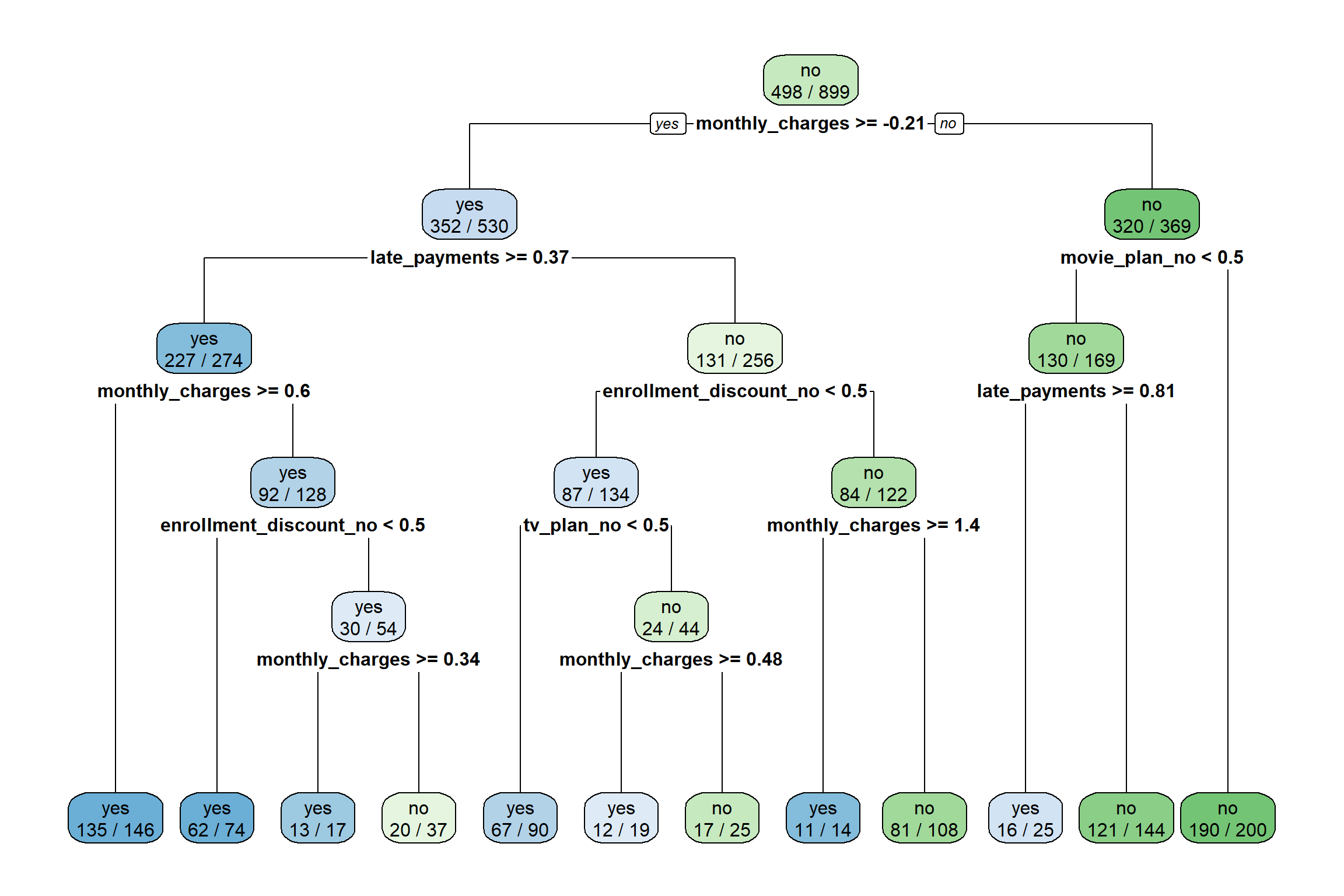

Train and Evaluate With `last_fit()`

Next we fit our final model workflow to the training data and evaluate performance on the test data.

The last_fit() function will fit our workflow to the training data and generate predictions on the test data as defined by our churn_split object.

tree_last_fit <- final_tree_workflow %>% 
                 last_fit(churn_split)

We can view our performance metrics on the test data

tree_last_fit %>% collect_metrics()

ROC Curve

We can plot the ROC curve to visualize test set performance of our tuned decision tree

tree_last_fit %>% collect_predictions() %>% 
                  roc_curve(truth  = churn, .pred_yes) %>% 
                  autoplot()

Confusion Matrix

We see that our model made 44 false negatives and 26 false positives on our test data set.

tree_predictions <- tree_last_fit %>% collect_predictions()

conf_mat(tree_predictions, truth = churn, estimate = .pred_class)

          Truth
Prediction yes  no
       yes  90  26
       no   44 141

Random Forests

In this section, we will fit a random forest model to the churn_df data. Random forests take decision trees and construct more powerful models in terms of prediction accuracy. The main mechanism that powers this algorithm is repeated sampling (with replacement) of the training data to produce a sequence of decision tree models. These models are then averaged to obtain a single prediction for a given value in the predictor space.

The random forest model selects a random subset of predictor variables for splitting the predictor space in the tree building process. This is done for every iteration of the algorithm, typically 100 to 2,000 times.

Data Spitting and Feature Engineering

We have already split our data into training, test, and cross validation sets as well as trained our feature engineering recipe, churn_recipe. These can be reused in our random forest workflow.

Model Specification

Next, we specify a random forest classifier with the following hyperparameters:

mtry: The number of predictors that will be randomly sampled at each split when creating the tree models
trees: The number of decision trees to fit and ultimately average
min_n: The minimum number of data points in a node that are required for the node to be split further

To specify a random forest model with tidymodels, we need the rand_forest() function. The hyperparameters of the model are arguments within the rand_forest() function and may be set to specific values. However, if tuning is required, then each of these parameters must be set to tune().

We will be using the ranger engine. This engine has an optional importance argument which can be used to track variable importance measures based on the Gini index. In order to make a variable importance plot with vip(), we must add importance = 'impurity' inside our set_engine() function.

rf_model <- rand_forest(mtry = tune(),
                        trees = tune(),
                        min_n = tune()) %>% 
            set_engine('ranger', importance = "impurity") %>% 
            set_mode('classification')

Workflow

Next, we combine our model and recipe into a workflow to easily manage the model-building process.

rf_workflow <- workflow() %>% 
               add_model(rf_model) %>% 
               add_recipe(churn_recipe)

Hyperparameter Tuning

Random Grid Search

We will perform a grid search on the random forest hyperparameters and select the best performing model based on the area under the ROC curve during cross validation.

In the previous section, we used grid_regular() to create a grid of hyperparameter values. This created a regualr grid of recommended default values.

Another way to do hyperparameter tuning is by creating a random grid of values. Many studies have shown that this method does better than the regular grid method.

Random grid search is implemented with the grid_random() function in tidymodels. Like grid_regular() it takes a sequence of hyperparameter names to create the grid. It also has a size parameter that specifies the number of random combinations to create.

The mtry() hyperparameter requires a pre-set range of values to test since it cannot exceed the number of columns in our data. When we add this to grid_random() we can pass mtry() into the range_set() function and set a range for the hyperparameter with a numeric vector.

In the code below, we set the range from 2 to 4. This is because we have 5 predictor variables in churn_df and we would like to test mtry() values somewhere in the middle between 1 and 5, trying to avoid values close to the ends.

When using grid_random(), it is suggested to use set.seed() for reproducability.

## Create a grid of hyperparameter values to test

set.seed(314)

rf_grid <- grid_random(mtry() %>% range_set(c(2, 4)),
                       trees(),
                       min_n(),
                       size = 10)

# View grid
rf_grid

Tuning Hyperparameters with `tune_grid()`

To find the optimal combination of hyperparameters from our tuning grid, we will use the tune_grid() function.

## Tune random forest workflow
set.seed(314)

rf_tuning <- rf_workflow %>% 
             tune_grid(resamples = churn_folds,
                       grid = rf_grid)

To view the results of our hyperparameter tuning, we can use the show_best() function. We must pass the type of performance metric we would like to see into the show_best() function.

## Show the top 5 best models based on roc_auc metric
rf_tuning %>% show_best('roc_auc')

## Select best model based on roc_auc
best_rf <- rf_tuning %>% 
           select_best(metric = 'roc_auc')

# View the best parameters
best_rf

Finalize Workflow

The last step in hyperparameter tuning is to use finalize_workflow() to add our optimal model to our workflow object.

final_rf_workflow <- rf_workflow %>% 
                     finalize_workflow(best_rf)

Variable Importance

In order to visualize the variable importance scores of our random forest model, we will need to manually train our workflow object with the fit() function.

Fit the Model

Next we fit our workflow to the training data. This is done by passing our workflow object to the fit() function.

rf_wf_fit <- final_rf_workflow %>% 
             fit(data = churn_training)

Once we have trained our model on our training data, we can study variable importance with the vip() function.

The first step is to extract the trained model from our workflow fit, rf_wf_fit. This can be done by passing rf_wf_fit to the extract_fit_parsnip() function.

rf_fit <- rf_wf_fit %>% 
          extract_fit_parsnip()

Variable Importance

Next we pass rf_fit to the vip() function. This will return a ggplot object with the variable importance scores from our model. The importance scores are based on the randomly chosen predictor variables, through the mtry() hyperparameter, that had the greatest predictive power.

We see from the results below, that monthly_charges by far is the most important predictor of churn.

vip(rf_fit)

Train and Evaluate With `last_fit()`

Next we fit our final model workflow to the training data and evaluate performance on the test data.

The last_fit() function will fit our workflow to the training data and generate predictions on the test data as defined by our churn_split object.

rf_last_fit <- final_rf_workflow %>% 
               last_fit(churn_split)

We can view our performance metrics on the test data

rf_last_fit %>% collect_metrics()

ROC Curve

We can plot the ROC curve to visualize test set performance of our random forest model.

rf_last_fit %>% collect_predictions() %>% 
                roc_curve(truth  = churn, .pred_yes) %>% 
                autoplot()

Confusion Matrix

We see that our model made 38 false negatives and 30 false positives on our test data set.

rf_predictions <- rf_last_fit %>% collect_predictions()

conf_mat(rf_predictions, truth = churn, estimate = .pred_class)

          Truth
Prediction yes  no
       yes  96  30
       no   38 137

Decision Trees and Random Forests

Data

Decision Trees

Data Splitting

Feature Engineering

Model Specification

Workflow

Hyperparameter Tuning

Tuning Hyperparameters with tune_grid()

Finalize Workflow

Visualize Results

Fit the Model

Exploring our Trained Model

Variable Importance

Decision Tree Plot

Train and Evaluate With last_fit()

ROC Curve

Confusion Matrix

Random Forests

Data Spitting and Feature Engineering

Model Specification

Workflow

Hyperparameter Tuning

Random Grid Search

Tuning Hyperparameters with tune_grid()

Finalize Workflow

Variable Importance

Fit the Model

Variable Importance

Train and Evaluate With last_fit()

ROC Curve

Confusion Matrix

Tuning Hyperparameters with `tune_grid()`

Train and Evaluate With `last_fit()`

Tuning Hyperparameters with `tune_grid()`

Train and Evaluate With `last_fit()`