Linear Regression with tidymodels
In this tutorial, we will learn about linear regression with
tidymodels. We will start by fitting a linear regression
model to the advertising data set that is used throughout
chapter 3 of our course textbook, An
Introduction to Statistical Learning.
Then we will focus on building our first machine learning pipeline,
with data resampling, featuring engineering, modeling fitting, and model
accuracy assessment using the workflows,
rsample, recipes, parsnip, and
tune packages from tidymodels.
Click the button below to clone the course R tutorials into your DataCamp Workspace. DataCamp Workspace is a free computation environment that allows for execution of R and Python notebooks. Note - you will only have to do this once since all tutorials are included in the DataCamp Workspace GBUS 738 project.
![]()
Introduction to Linear Regression
The R code below will load the data and packages we will
be working with throughout this tutorial. The vip package
is used for exploring predictor variable importance. We will use this
package for visualizing which predictors have the most predictive power
in our linear regression models.
# Load libraries
library(tidymodels)
library(vip) # for variable importance

# Load data sets
advertising <- readRDS(url('https://gmubusinessanalytics.netlify.app/data/advertising.rds'))

home_sales <- readRDS(url('https://gmubusinessanalytics.netlify.app/data/home_sales.rds')) %>%
              select(-selling_date)
Data
We will be working with the advertisting data set, where
each row represents a store from a large retail chain and their
associated sales revenue and advertising budgets, and the
home_sales data, where each row represents a real estate
home sale in the Seattle area between 2014 and 2015.
Take a moment to explore these data sets below.
Advertising Data
Seattle Home Sales
Data Splitting
The first step in building regression models is to split our original data into a training and test set. We then perform all feature engineering and model fitting tasks on the training set and use the test set as an independent assessment of our model’s prediction accuracy.
We will be using the initial_split() function from
rsample to partition the advertising data into
training and test sets. Remember to always use set.seed()
to ensure your results are reproducible.
set.seed(314)

# Create a split object
advertising_split <- initial_split(advertising, prop = 0.75,
                                   strata = Sales)

# Build training data set
advertising_training <- advertising_split %>%
                        training()

# Build testing data set
advertising_test <- advertising_split %>%
                    testing()
Model Specification
The next step in the process is to build a linear regression model object to which we fit our training data.
For every model type, such as linear regression, there are numerous
packages (or engines) in R that can be used.
For example, we can use the lm() function from base
R or the stan_glm() function from the
rstanarm package. Both of these functions will fit a linear
regression model to our data with slightly different
implementations.
The parsnip package from tidymodels acts
like an aggregator across the various modeling engines within
R. This makes it easy to implement machine learning
algorithms from different R packages with one unifying
syntax.
To specify a model object with parsnip, we must:
- Pick a model type
- Set the engine
- Set the mode (either regression or classification)
Linear regression is implemented with the linear_reg()
function in parsnip. To the set the engine and mode, we use
set_engine() and set_mode() respectively. Each
one of these functions takes a parsnip object as an argument and updates
its properties.
To explore all parsnip models, please see the documentation where you can search by keyword.
Let’s create a linear regression model object with the
lm engine. This is the default engine for most
applications.
lm_model <- linear_reg() %>%
            set_engine('lm') %>% # adds lm implementation of linear regression
            set_mode('regression')

# View object properties
lm_model
Linear Regression Model Specification (regression)
Computational engine: lm
Fitting to Training Data
Now we are ready to train our model object on the
advertising_training data. We can do this using the
fit() function from the parsnip package. The
fit() function takes the following arguments:
- a
parnsipmodel object specification - a model formula
- a data frame with the training data
The code below trains our linear regression model on the
advertising_training data. In our formula, we have
specified that Sales is the response variable and
TV, Radio, and Newspaper are our
predictor variables.
We have assigned the name lm_fit to our trained linear
regression model.
lm_fit <- lm_model %>%
          fit(Sales ~ ., data = advertising_training)

# View lm_fit properties
lm_fit
parsnip model object
Call:
stats::lm(formula = Sales ~ ., data = data)
Coefficients:
(Intercept) TV Radio Newspaper
2.90436 0.04597 0.18432 0.00237
Exploring Training Results
As mentioned in the first R tutorial, most model objects in
R are stored as specialized lists.
The lm_fit object is list that contains all of the
information about how our model was trained as well as the detailed
results. Let’s use the names() function to print the named
objects that are stored within lm_fit.
The important objects are fit and preproc.
These contain the trained model and pre-processing steps (if any are
used), respectively.
names(lm_fit)[1] "lvl" "spec" "fit" "preproc" "elapsed"
[6] "censor_probs"
To print a summary of our model, we can extract fit from
lm_fit and pass it to the summary() function.
We can explore the estimated coefficients, F-statistics, p-values,
residual standard error (also known as RMSE) and R2 value.
However, this feature is best for visually exploring our results on the training data since the results are not returned as a data frame. In the coming sections, we will explore numerous functions that can automatically extract this information from a linear regression results object.
Below, we use the pluck() function from
dplyr to extract the fitresults from
lm_fit. This is the same as using lm_fit$fit
or lm_fit[['fit']].
lm_fit %>%
  # Extract fit element from the list
  pluck('fit') %>%
  # Pass to summary function
  summary()
Call:
stats::lm(formula = Sales ~ ., data = data)

Residuals:
   Min     1Q Median     3Q    Max
-8.656 -0.902  0.247  1.249  2.801

Coefficients:
            Estimate Std. Error t value Pr(>|t|)
(Intercept)  2.90436    0.38649    7.51  5.5e-12 ***
TV           0.04597    0.00173   26.57  < 2e-16 ***
Radio        0.18432    0.01018   18.11  < 2e-16 ***
Newspaper    0.00237    0.00709    0.33     0.74
---
Signif. codes:  0 '***' 0.001 '**' 0.01 '*' 0.05 '.' 0.1 ' ' 1

Residual standard error: 1.8 on 144 degrees of freedom
Multiple R-squared:  0.887, Adjusted R-squared:  0.884
F-statistic:  375 on 3 and 144 DF,  p-value: <2e-16
We can use the plot() function to obtain diagnostic
plots for our trained regression model. Again, we must first extract the
fit object from lm_fit and then pass it into
plot(). These plots provide a check for the main
assumptions of the linear regression model.
par(mfrow=c(2,2)) # plot all 4 plots in one

lm_fit %>%
  pluck('fit') %>%
  plot(pch = 16,    # optional parameters to make points blue
       col = '#006EA1')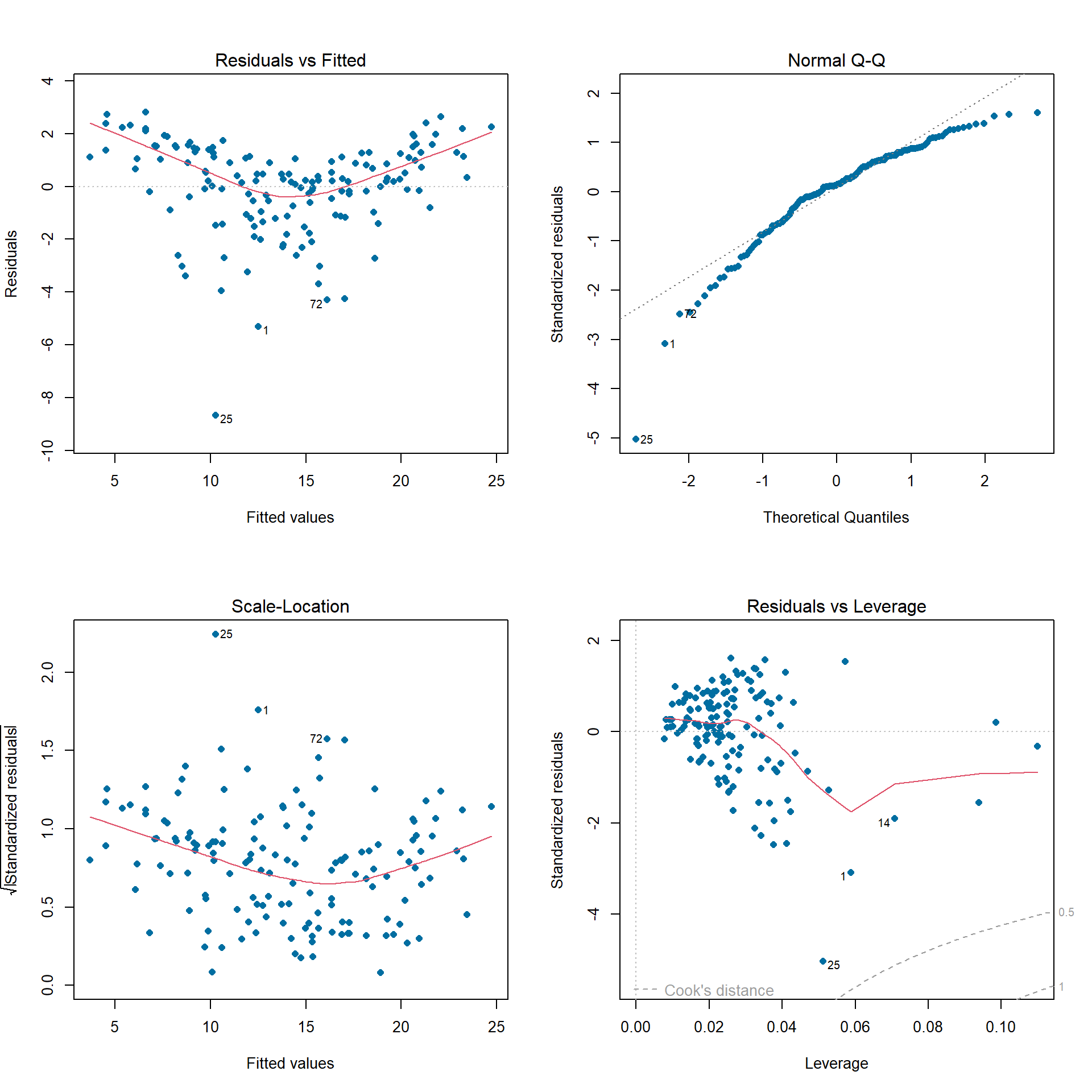
Tidy Training Results
To obtain the detailed results from our trained linear regression
model in a data frame, we can use the tidy() and
glance() functions directly on our trained
parsnip model, lm_fit.
The tidy() function takes a linear regression object and
returns a data frame of the estimated model coefficients and their
associated F-statistics and p-values.
The glance() function will return performance metrics
obtained on the training data such as the R2 value
(r.squared) and the RMSE (sigma).
# Data frame of estimated coefficients
tidy(lm_fit)
# Performance metrics on training data
glance(lm_fit)
We can also use the vip() function to plot the variable
importance for each predictor in our model. The importance value is
determined based on the F-statistics and estimate coefficents in our
trained model object.
vip(lm_fit)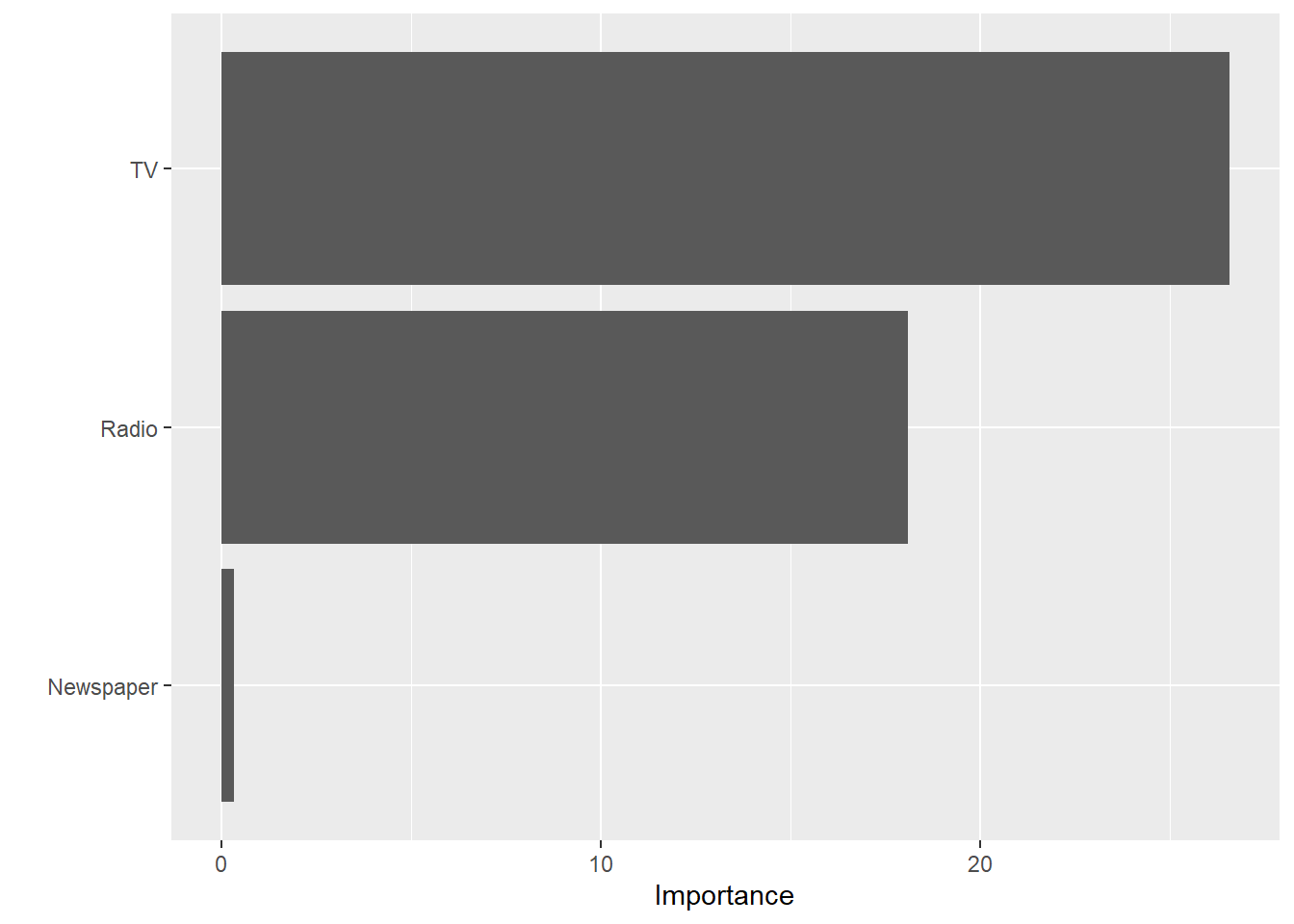
Evaluating Test Set Accuracy
To assess the accuracy of our trained linear regression model,
lm_fit, we must use it to make predictions on our test
data, advertising_test.
This is done with the predict() function from
parnsip. This function takes two important arguments:
- a trained
parnsipmodel object new_datafor which to generate predictions
The code below uses the predict function to generate a
data frame with a single column, .pred, which contains the
predicted Sales values on the
advertisting_test data.
predict(lm_fit, new_data = advertising_test)
Generally it’s best to combine the test data set and the predictions
into a single data frame. We create a data frame with the predictions on
the advertising_test data and then use
bind_cols to add the advertising_test data to
the results.
Now we have the model results and the test data in a single data
frame.
advertising_test_results <- predict(lm_fit, new_data = advertising_test) %>%
                            bind_cols(advertising_test)

# View results
advertising_test_results
Calculating RMSE and R2 on the Test Data
To obtain the RMSE and R2 values on our test set results,
we can use the rmse() and rsq() functions.
Both functions take the following arguments:
data- a data frame with columns that have the true values and predictionstruth- the column with the true response valuesestimate- the column with predicted values
In the examples below we pass our
advertising_test_results to these functions to obtain these
values for our test set. results are always returned as a data frame
with the following columns: .metric,
.estimator, and .estimate.
# RMSE on test set
rmse(advertising_test_results,
     truth = Sales,
     estimate = .pred)
# R2 on test set
rsq(advertising_test_results,
    truth = Sales,
    estimate = .pred)
R2 Plot
The best way to assess the test set accuracy is by making an R2 plot. This is a plot that can be used for any regression model.
It plots the actual values (Sales) versus the model
predictions (.pred) as a scatter plot. It also plot the
line y = x through the origin. This line is a visually
representation of the perfect model where all predicted values are equal
to the true values in the test set. The farther the points are from this
line, the worse the model fit.
The reason this plot is called an R2 plot, is because the R2 is simply the squared correlation between the true and predicted values, which are plotted as paired in the plot.
In the code below, we use geom_point() and
geom_abline() to make this plot using out
advertising_test_results data. The
geom_abline() function will plot a line with the provided
slope and intercept arguments. The
coord_obs_pred() function scales the x and y axis to have
the same range for accurate comparisons.
ggplot(data = advertising_test_results,
       mapping = aes(x = .pred, y = Sales)) +
  geom_point(alpha = 0.4) +
  geom_abline(intercept = 0, slope = 1, linetype = 2, color = 'red') +
  coord_obs_pred() +
  labs(title = 'Linear Regression Results - Advertising Test Set',
       x = 'Predicted Sales',
       y = 'Actual Sales') +
  theme_light()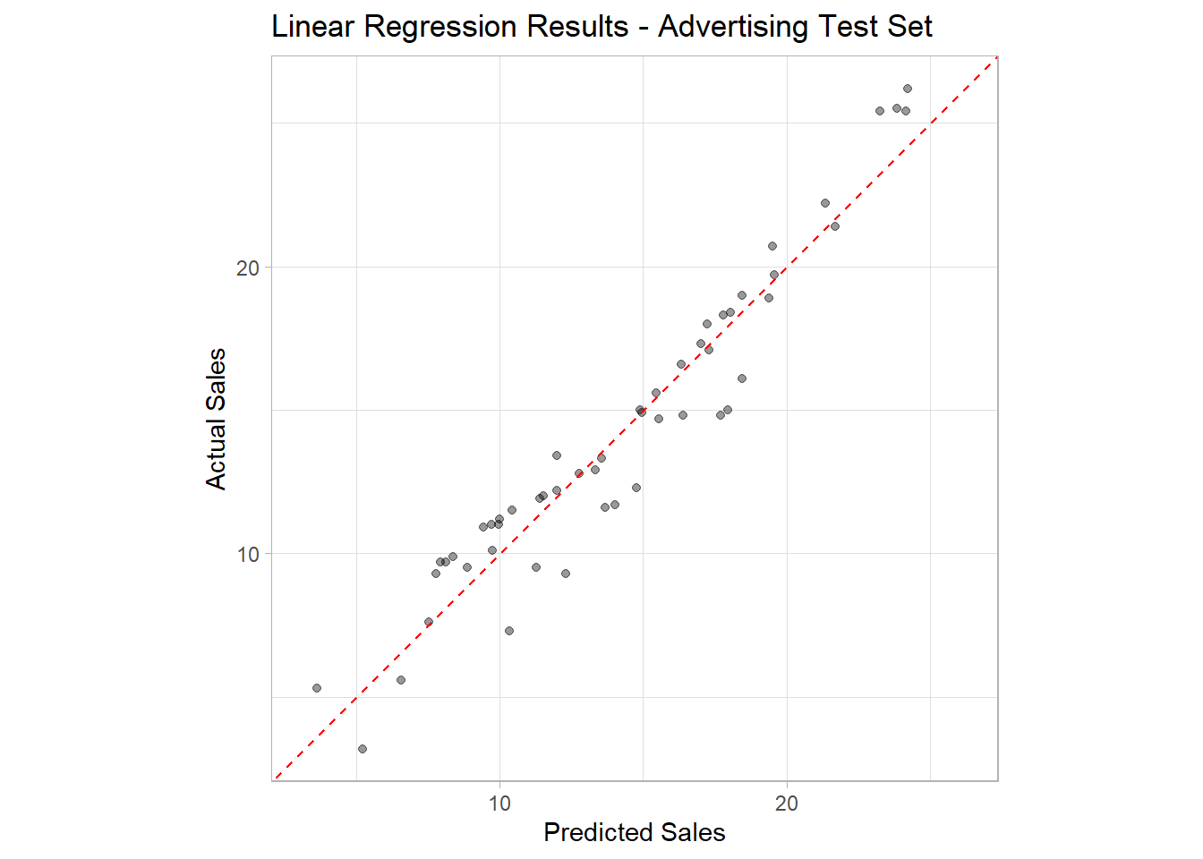
Creating a Machine Learning Workflow
In the previous section, we trained a linear regression model to the
advertising data step-by-step. In this section, we will go
over how to combine all of the modeling steps into a single
workflow.
We will be using the workflow package, which combines a
parnsip model with a recipe, and the
last_fit() function to build an end-to-end modeling
training pipeline.
Let’s assume we would like to do the following with the
advertising data:
- Split our data into training and test sets
- Feature engineer the training data by removing skewness and normalizing numeric predictors
- Specify a linear regression model
- Train our model on the training data
- Transform the test data with steps learned in part 2 and obtain predictions using our trained model
The machine learning workflow can be accomplished with a few
steps using tidymodels
Step 1. Split Our Data
First we split our data into training and test sets.
set.seed(314)

# Create a split object
advertising_split <- initial_split(advertising, prop = 0.75,
                                   strata = Sales)

# Build training data set
advertising_training <- advertising_split %>%
                        training()

# Build testing data set
advertising_test <- advertising_split %>%
                    testing()
Step 2. Feature Engineering
Next, we specify our feature engineering recipe. In this step, we
do not use prep() or bake().
This recipe will be automatically applied in a later step using the
workflow() and last_fit() functions.
advertising_recipe <- recipe(Sales ~ ., data = advertising_training) %>%
                      step_YeoJohnson(all_numeric(), -all_outcomes()) %>%
                      step_normalize(all_numeric(), -all_outcomes())
Step 3. Specify a Model
Next, we specify our linear regression model with
parsnip.
lm_model <- linear_reg() %>%
            set_engine('lm') %>%
            set_mode('regression')
Step 4. Create a Workflow
The workflow package was designed to combine models and
recipes into a single object. To create a workflow, we start with
workflow() to create an empty workflow and then add out
model and recipe with add_model() and
add_recipe().
advertising_workflow <- workflow() %>%
                        add_model(lm_model) %>%
                        add_recipe(advertising_recipe)
Step 5. Execute the Workflow
The last_fit() function will take a workflow object and
apply the recipe and model to a specified data split object.
In the code below, we pass the advertising_workflow
object and advertising_split object into
last_fit().
The last_fit() function will then train the feature
engineering steps on the training data, fit the model to the training
data, apply the feature engineering steps to the test data, and
calculate the predictions on the test data, all in one
step!
advertising_fit <- advertising_workflow %>%
                   last_fit(split = advertising_split)
To obtain the performance metrics and predictions on the test set, we
use the collect_metrics() and
collect_predictions() functions on our
advertising_fit object.
# Obtain performance metrics on test data
advertising_fit %>% collect_metrics()
We can save the test set predictions by using the
collect_predictions() function. This function returns a
data frame which will have the response variables values from the test
set and a column named .pred with the model
predictions.
# Obtain test set predictions data frame
test_results <- advertising_fit %>%
                collect_predictions()
# View results
test_results
Workflow for Home Selling Price
For another example of fitting a machine learning workflow, let’s use
linear regression to predict the selling price of homes using the
home_sales data.
For our feature engineering steps, we will include removing skewness
and normalizing numeric predictors, and creating dummy variables for the
city variable.
Remember that all machine learning algorithms need a numeric feature matrix. Therefore we must also transform character or factor predictor variables to dummy variables.
Step 1. Split Our Data
First we split our data into training and test sets.
set.seed(271)

# Create a split object
homes_split <- initial_split(home_sales, prop = 0.75,
                             strata = selling_price)

# Build training data set
homes_training <- homes_split %>%
                  training()

# Build testing data set
homes_test <- homes_split %>%
              testing()
Step 2. Feature Engineering
Next, we specify our feature engineering recipe. In this step, we
do not use prep() or bake().
This recipe will be automatically applied in a later step using the
workflow() and last_fit() functions.
For our model formula, we are specifying that
selling_price is our response variable and all others are
predictor variables.
homes_recipe <- recipe(selling_price ~ ., data = homes_training) %>%
                step_YeoJohnson(all_numeric(), -all_outcomes()) %>%
                step_normalize(all_numeric(), -all_outcomes()) %>%
                step_dummy(all_nominal(), - all_outcomes())
As an intermediate step, let’s check our recipe by prepping it on the training data and applying it to the test data. We want to make sure that we get the correct transformations.
From the results below, things look correct.
homes_recipe %>%
  prep(training = homes_training) %>%
  bake(new_data = homes_test)
Step 3. Specify a Model
Next, we specify our linear regression model with
parsnip.
lm_model <- linear_reg() %>%
            set_engine('lm') %>%
            set_mode('regression')
Step 4. Create a Workflow
Next, we combine our model and recipe into a workflow object.
homes_workflow <- workflow() %>%
                  add_model(lm_model) %>%
                  add_recipe(homes_recipe)
Step 5. Execute the Workflow
Finally, we process our machine learning workflow with
last_fit().
homes_fit <- homes_workflow %>%
             last_fit(split = homes_split)
To obtain the performance metrics and predictions on the test set, we
use the collect_metrics() and
collect_predictions() functions on our
homes_fit object.
# Obtain performance metrics on test data
homes_fit %>%
  collect_metrics()
We can save the test set predictions by using the
collect_predictions() function. This function returns a
data frame which will have the response variables values from the test
set and a column named .pred with the model
predictions.
# Obtain test set predictions data frame
homes_results <- homes_fit %>%
                 collect_predictions()
# View results
homes_results
R2 Plot
Finally, let’s use the homes_results data frame to make
an R2 plot to visualize our model performance on the test
data set.
ggplot(data = homes_results,
       mapping = aes(x = .pred, y = selling_price)) +
  geom_point(alpha = 0.2) +
  geom_abline(intercept = 0, slope = 1, color = 'red', linetype = 2) +
  coord_obs_pred() +
  labs(title = 'Linear Regression Results - Home Sales Test Set',
       x = 'Predicted Selling Price',
       y = 'Actual Selling Price') +
  theme_light()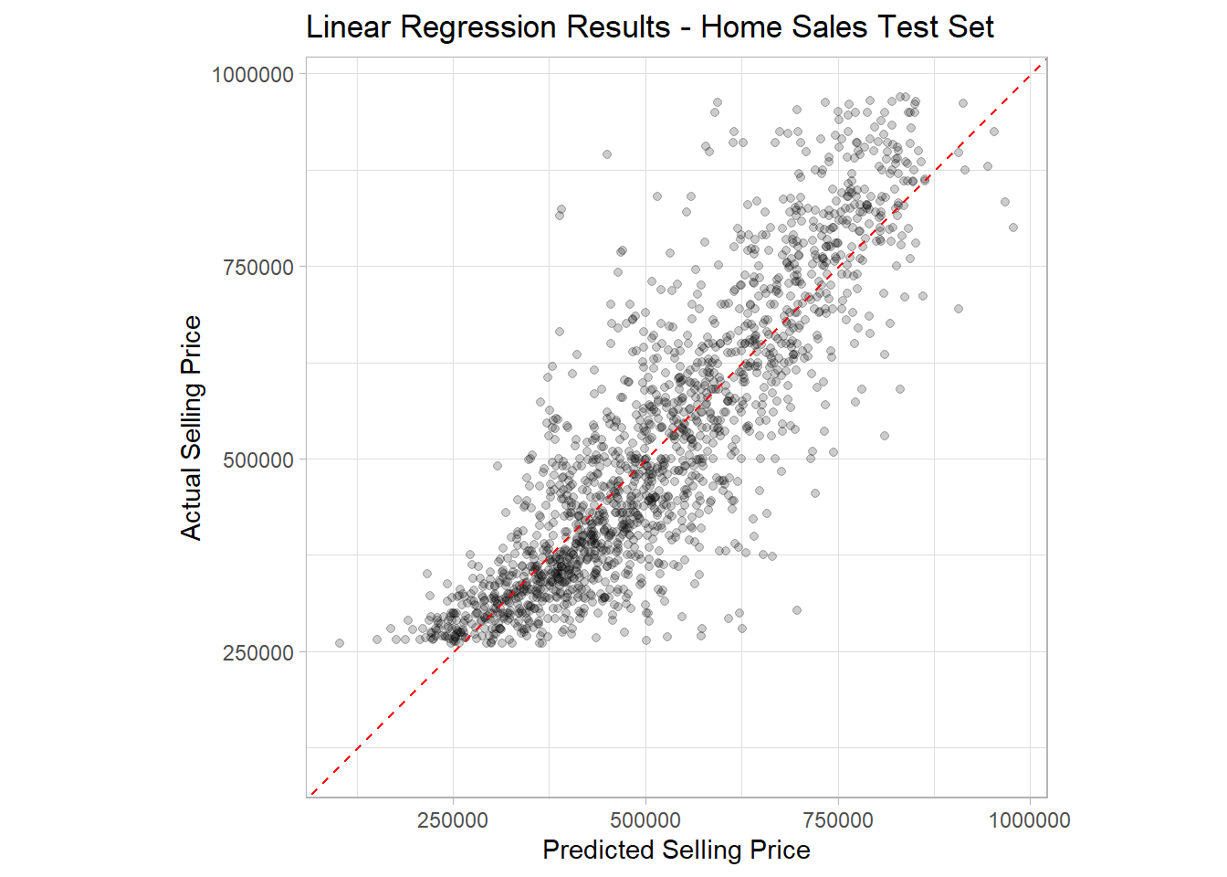
Variable Importance
Creating a workflow and using the last_fit() function is
a great option of automating a machine learning
pipeline. However, we are not able to explore variable importance on the
training data when we fit our model with last_fit().
To obtain a variable importance plot with vip(), we must
use the methods introduced at the beginning of the tutorial. This
involves fitting the model with the fit() function on the
training data.
To do this, we will train our homes_recipe and transform
our training data. Then we use the fit() function to train
our linear regression object, lm_model, on our processed
data.
Then we can use the vip() function to see which
predictors were most important.
homes_training_baked <- homes_recipe %>%
                        prep(training = homes_training) %>%
                        bake(new_data = NULL)

# View results
homes_training_baked
Now we fit our linear regression model to the baked training data.
homes_lm_fit <- lm_model %>%
                fit(selling_price ~ ., data = homes_training_baked)
Finally, we use vip() on our trained linear regression
model. It appears that square footage and location are the most
importance predictor variables.
vip(homes_lm_fit)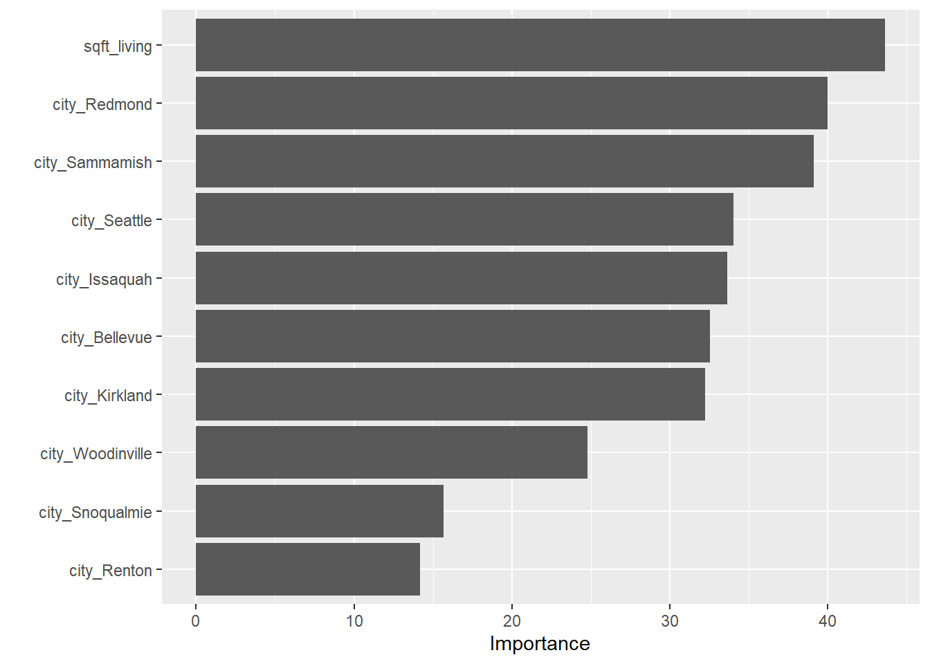
Copyright © David Svancer 2023 |