Data

Logistic Regression

Data Splitting
Feature Engineering
Check Transformations
Specify Logistic Regression Model
Create a Workflow
Fit Model
Collect Predictions
Evaluate Model Performance

Linear Discriminant Analysis

Specify LDA model
Create LDA Workflow
Fit Model
Collect Predictions
Evaluate Model Performance

KNN Classification

Specify KNN model
Create KNN Workflow
Tune Hyperparameter
Fit Model
Collect Predictions
Evaluate Model Performance

The goal of this tutorial is to provide solved examples of model-fitting with tidymodels to help you solidify your learning from the R tutorials.

Data

The R code chunk below will load the tidymodels and discrim packages as well as the mobile_carrier_df data set.

library(tidymodels)
library(discrim)

mobile_carrier_df <- 
  readRDS(url('https://gmubusinessanalytics.netlify.app/data/mobile_carrier_data.rds'))

The mobile_carrier_df data frame contains information on U.S. customers for a national mobile service carrier.

Each row represents a customer who did or did not cancel their service. The response variable in this data set is named canceled_plan and has levels of ‘yes’ or ‘no’. The predictor variables in this data frame contain information about the customers’ residence region and mobile call activity.

Our goal is to predict canceled_plan with various machine learning algorithms including logistic regression, LDA, and KNN.

mobile_carrier_df

ABCDEFGHIJ0123456789

canceled_plan <fct>	us_state_region <fct>	international_plan <fct>	voice_mail_plan <fct>
yes	East North Central	no	no
no	South Atlantic	no	yes
yes	New England	no	no
no	South Atlantic	no	no
no	Mountain	no	yes
yes	East North Central	no	no
no	East South Central	no	yes
yes	Mid Atlantic	yes	no
no	Mountain	yes	yes
no	South Atlantic	no	no

Logistic Regression

Data Splitting

set.seed(271)

mobile_split <- initial_split(mobile_carrier_df, prop = 0.75,
                              strata = canceled_plan)

mobile_training <- mobile_split %>% 
                   training()

mobile_test <- mobile_split %>%
               testing()


# Create cross validation folds for hyperparameter tuning
set.seed(271)

mobile_folds <- vfold_cv(mobile_training, v = 5)

Feature Engineering

We create a feature engineering pipeline, mobile_recipe, with the following transformations:

Remove skewness from numeric predictors
Normalize all numeric predictors
Create dummy variables for all nominal predictors

mobile_recipe <- recipe(canceled_plan ~ ., data = mobile_training) %>% 
                 step_YeoJohnson(all_numeric(), -all_outcomes()) %>% 
                 step_normalize(all_numeric(), -all_outcomes()) %>% 
                 step_dummy(all_nominal(), -all_outcomes())

Check Transformations

It’s always good practice to check your transformations by applying them to the training data.

mobile_recipe %>% 
  prep(training = mobile_training) %>% 
  bake(new_data = NULL)

ABCDEFGHIJ0123456789

number_vmail_messages <dbl>	total_day_minutes <dbl>	total_day_calls <dbl>	total_eve_minutes <dbl>
-0.5737528	-0.7961420163	0.31432134	1.0665306242
1.7541177	0.7390979014	-0.75175966	0.9165627874
1.7440365	0.6230319393	0.81394217	-0.9326572335
-0.5737528	-0.0413027110	0.01887266	0.1924920726
-0.5737528	-0.2494271001	-0.65687950	0.2773575238
-0.5737528	0.5910140026	0.56303561	0.4565155630
-0.5737528	-0.3306291677	-1.44883535	1.5162521376
-0.5737528	-0.9141890845	0.11698262	1.5065922239
1.7681880	-0.3687107675	-1.49433811	1.3537800818
-0.5737528	-1.2574122978	1.11781889	1.5143202655

Specify Logistic Regression Model

Next, we specify a logistic regression model using the appropriate parnsip function.

logistic_model <- logistic_reg() %>% 
                  set_engine('glm') %>% 
                  set_mode('classification')

Create a Workflow

Next, we combine our model and recipe into a single workflow, logistic_wf

logistic_wf <- workflow() %>% 
               add_model(logistic_model) %>% 
               add_recipe(mobile_recipe)

Fit Model

Next, we fit our workflow using the last_fit() function. This will train our model on the training data and calculate predictions on the test data.

logistic_fit <- logistic_wf %>% 
                last_fit(split = mobile_split)

Collect Predictions

The collect_predictions() creates a data frame of test results.

logistic_results <-  logistic_fit %>% 
                     collect_predictions()

Evaluate Model Performance

Next we calculate the ROC Curve, area under the ROC curve, and the confusion matrix on the test data.

Results

## ROC Curve
roc_curve(logistic_results, 
          truth = canceled_plan, 
          .pred_yes) %>% 
  autoplot()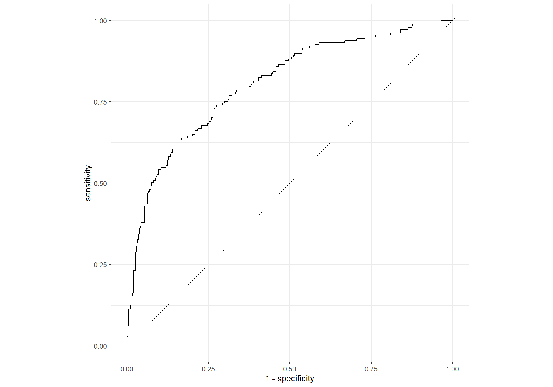

# ROC AUC
roc_auc(logistic_results, 
        truth = canceled_plan,
        .pred_yes)

ABCDEFGHIJ0123456789

.metric <chr>	.estimator <chr>	.estimate <dbl>
roc_auc	binary	0.8050488

# Confusion Matrix
conf_mat(logistic_results, 
         truth = canceled_plan, 
         estimate = .pred_class)

          Truth
Prediction yes  no
       yes  90  34
       no   87 359

Linear Discriminant Analysis

In this section we will modify the steps from above to fit an LDA model to the mobile_carrier_df data. We have already created our training/test/data folds and trained our feature engineering recipe.

To fit an LDA model, we must specify an LDA object with discrim_regularized(), create an LDA workflow, and fit our model with last_fit().

Specify LDA model

lda_model <- discrim_regularized(frac_common_cov = 1) %>% 
             set_engine('klaR') %>% 
             set_mode('classification')

Create LDA Workflow

lda_wf <- workflow() %>% 
          add_model(lda_model) %>% 
          add_recipe(mobile_recipe)

Fit Model

lda_fit <- lda_wf %>% 
           last_fit(split = mobile_split)

Collect Predictions

Use the collect_predictions() function to create a data frame of test results.

lda_results <-  lda_fit %>% 
                collect_predictions()

Evaluate Model Performance

Calculate the ROC Curve, area under the ROC curve, and the confusion matrix on the test data. You should get the results below.

Results

## ROC Curve
roc_curve(lda_results, 
          truth = canceled_plan, 
          .pred_yes) %>% 
  autoplot()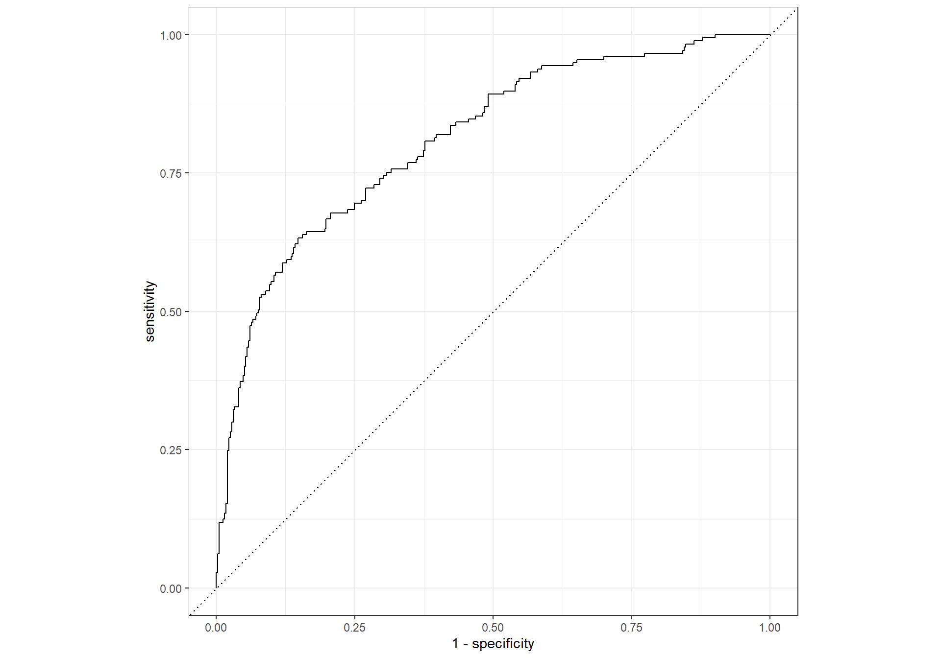

# ROC AUC
roc_auc(lda_results, 
        truth = canceled_plan, 
        .pred_yes)

ABCDEFGHIJ0123456789

.metric <chr>	.estimator <chr>	.estimate <dbl>
roc_auc	binary	0.810181

# Confusion Matrix
conf_mat(lda_results, 
         truth = canceled_plan, 
         estimate = .pred_class)

          Truth
Prediction yes  no
       yes  87  29
       no   90 364

KNN Classification

In this section we will modify the steps from above to fit an KNN model to the mobile_carrier_df data.

To fit a KNN model, we must specify an KNN object with nearest_neighbor(), create a KNN workflow, tune our hyperparameter, neighbors, and fit our model with last_fit().

Specify KNN model

knn_model <- nearest_neighbor(neighbors = tune()) %>% 
             set_engine('kknn') %>% 
             set_mode('classification')

Create KNN Workflow

knn_wf <- workflow() %>% 
          add_model(knn_model) %>% 
          add_recipe(mobile_recipe)

Tune Hyperparameter

Create Tuning Grid

Next, we create a grid of the following values of neighbors: 10, 15, 25, 45, 60, 80, 100, 120, 140, and 180

## Create a grid of hyperparameter values to test
k_grid <- tibble(neighbors = c(10, 15, 25, 45, 60, 80, 100, 120, 140, 180))

Grid Search

Next, we use tune_grid() to perform hyperparameter tuning using k_grid and mobile_folds.

## Tune  workflow
set.seed(314)

knn_tuning <- knn_wf %>% 
              tune_grid(resamples = mobile_folds,
                        grid = k_grid)

Select Best Model

The select_best() function selects the best model from our tuning results based on the area under the ROC curve.

## Select best model based on roc_auc
best_k <- knn_tuning %>% 
          select_best(metric = 'roc_auc')

Finalize Workflow

The last step is to use finalize_workflow() to add our optimal model to our workflow object.

## Finalize workflow by adding the best performing model

final_knn_wf <- knn_wf %>% 
                finalize_workflow(best_k)

Fit Model

knn_fit <- final_knn_wf %>% 
           last_fit(split = mobile_split)

Collect Predictions

Use the collect_predictions() function to create a data frame of test results.

knn_results <-  knn_fit %>% 
                collect_predictions()

Evaluate Model Performance

Calculate the ROC Curve, area under the ROC curve, and the confusion matrix on the test data. You should get the results below.

Results

## ROC Curve
roc_curve(knn_results, 
          truth = canceled_plan, 
          .pred_yes) %>% 
  autoplot()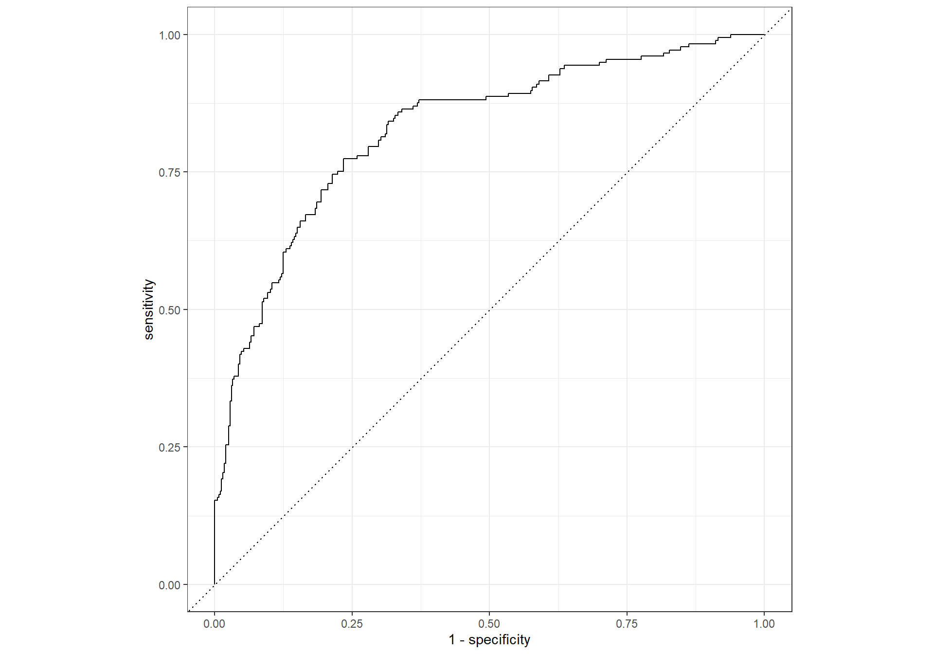

# ROC AUC
roc_auc(knn_results, 
        truth = canceled_plan, 
        .pred_yes)

ABCDEFGHIJ0123456789

.metric <chr>	.estimator <chr>	.estimate <dbl>
roc_auc	binary	0.8272164

# Confusion Matrix
conf_mat(knn_results, 
         truth = canceled_plan, 
         estimate = .pred_class)

          Truth
Prediction yes  no
       yes   9   0
       no  168 393

Machine Learning with tidymodels

Data

Logistic Regression

Data Splitting

Feature Engineering

Check Transformations

Specify Logistic Regression Model

Create a Workflow

Fit Model

Collect Predictions

Evaluate Model Performance

Results

Linear Discriminant Analysis

Specify LDA model

Create LDA Workflow

Fit Model

Collect Predictions

Evaluate Model Performance

Results

KNN Classification

Specify KNN model

Create KNN Workflow

Tune Hyperparameter

Create Tuning Grid

Grid Search

Select Best Model

Finalize Workflow

Fit Model

Collect Predictions

Evaluate Model Performance

Results